Part 1 - AM transmitters

Objectives

This lab is a guide to AM signal waveforms. In this part you will learn:

Theory and equations of AM signals and the complex mixer
How to construct an AM transmitter flowgraph to generate an AM waveform with a sinusoidal message and observe the waveform and spectrum
Construction of AM transmitter flowgraphs with square wave and pseudo-random data messages

Part 1 Deliverables

GRC files of AM transmitter and waveform builder. You will be stepped through building them. They will be named:
- waveform_builder.grc
- AM_modulator.grc
There are 2 questions spaced throughout this part. They are clearly indicated.
- Each question requires approximately 1 line of writing, and address concepts, not details. Answer the questions and submit a single page containing the answers to your TA at the end of the lab.

Building an AM transmitter

Review AM transmitter theory in the textbook (section 2.1).
If you are unsure of the functionality of any of the blocks, please consult the Documentation, or ask your TA.

To begin, start GRC as was done in the intro tutorials. If GRC is already open, open the .grc files by selecting File->Open, or clicking on the Open logo, .

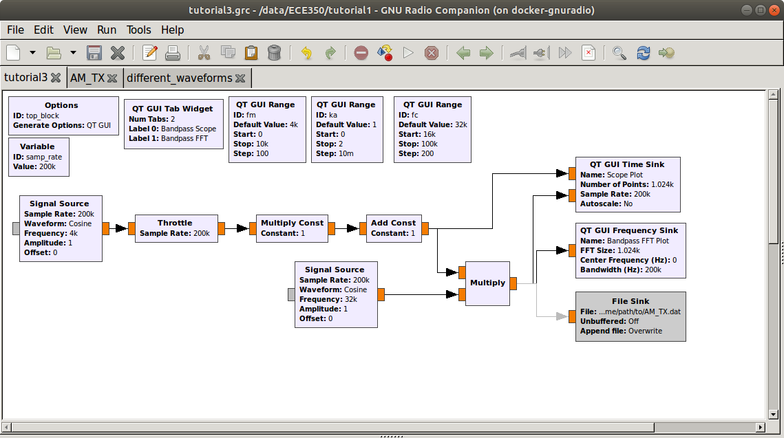
Build the following flowgraph using Signal Source, Throttle, Multiply Const, and Add Const blocks. It would be wise to have the different GUI sinks in different window tabs as done in the second intro tutorial.

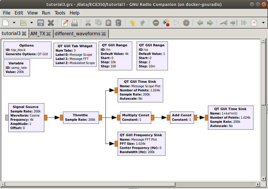
AM modulation flow graph

This flowgraph will be one of your deliverables. Save it as AM_modulator.grc and in the Options block, set the following parameters as follows.

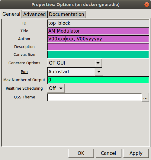
Flowgraph options parameters for submission

You can read the QT GUI Range widget parameters right off of the flowgraph, and note that the sample rate is 200 kHz. You cannot however, tell when variables are in use without opening the blocks.

The two blocks using the QT GUI Range variables are the Signal Source and the Multiply Const. Use the following two figures as references.
Set the Add Const constant to 1.
You can name and organize the GUI sinks/scopes as you please. Don’t forget to set Config->Control Panel to “Yes” in the GUI sinks to allow interactivity.

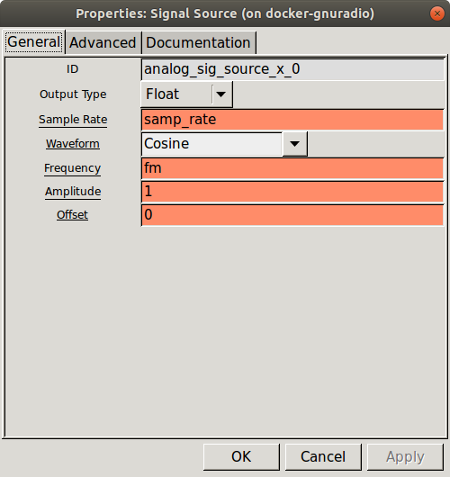
Signal source properties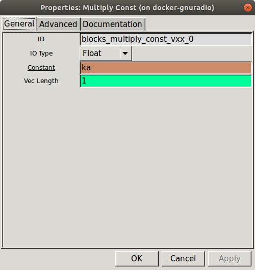

Multiple const properties properties

Note

This flowgraph is the graphical form of the modulation waveform, \(1+k_a * m(t)\), where \(m(t)\) is the Signal Source block, 1 is the Add Const block, and \(k_a\) is the Multiply Const block.

When executed, the three plots should look like the following:

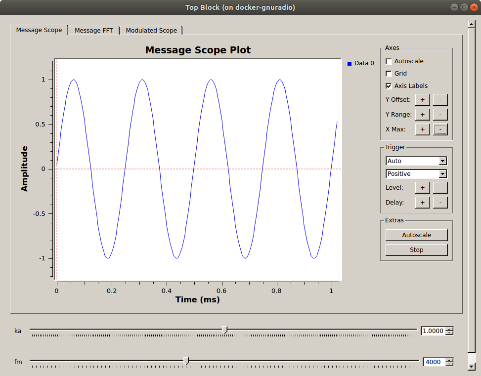
Message in time domain

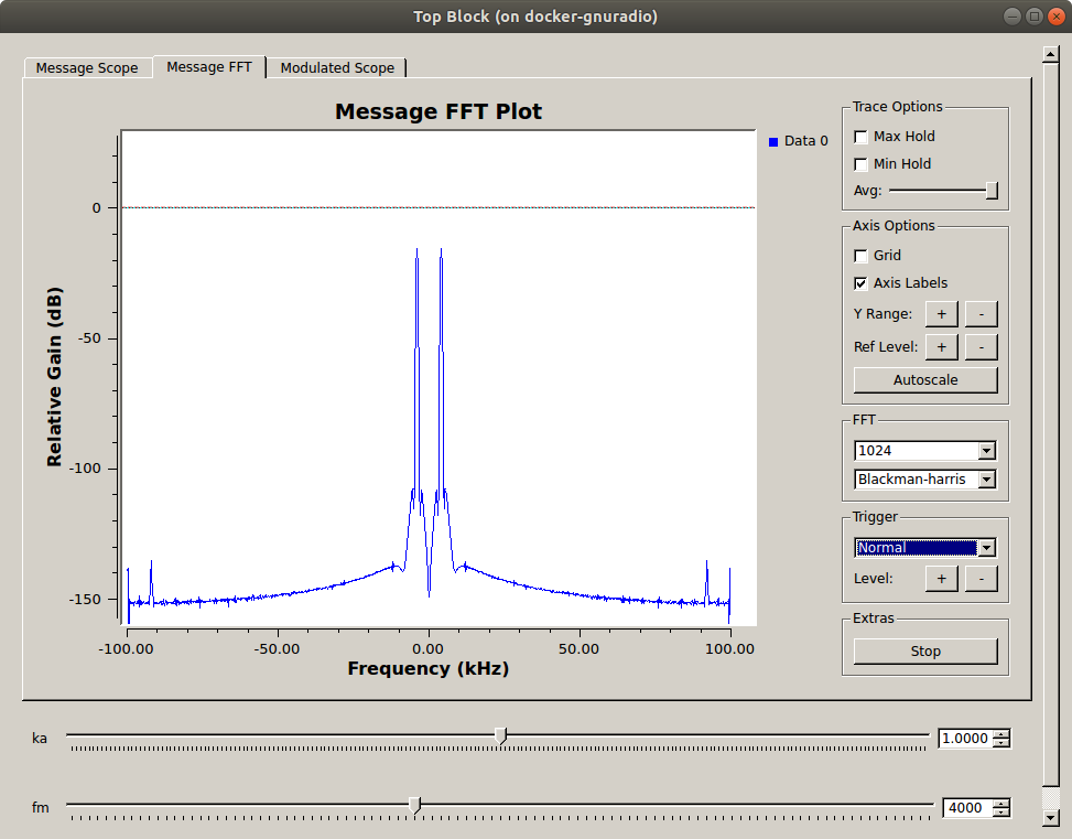
Message in frequency domain

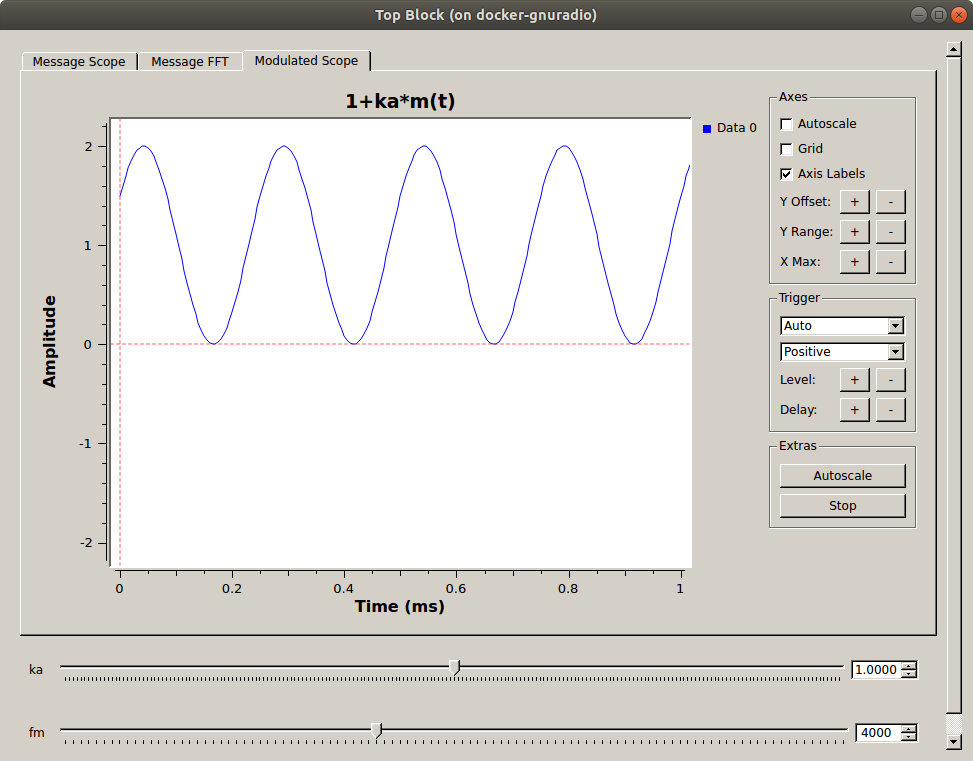
Modulation signal in time domain

Deliverable Question 1

Why is the spectrum symmetrical about 0 Hz?

Now multiply the modulation waveform with the carrier signal to obtain the AM modulated waveform. Note the added QT GUI Range widget for \(f_c\).

Set the carrier signal source block frequency to fc.
In the QT GUI Range widget for the fc variable, set the maximum value as samp_rate/2
In the QT GUI Time Sink:
- change the number of inputs to two as shown, and connect one to each of the modulation waveform and the modulated carrier.
- go to the Config tab and label the two lines as “Modulation waveform” and “Modulated signal” as appropriate.
Flowgraph of AM modulation with a carrier

Note

In GNU Radio Companion, greyed out boxes are ‘disabled. You can do this by right clicking on a block and selecting ‘Disable’, or just pressing the ‘d’ key on your keyboard. They greyed out File Sink will be used later.

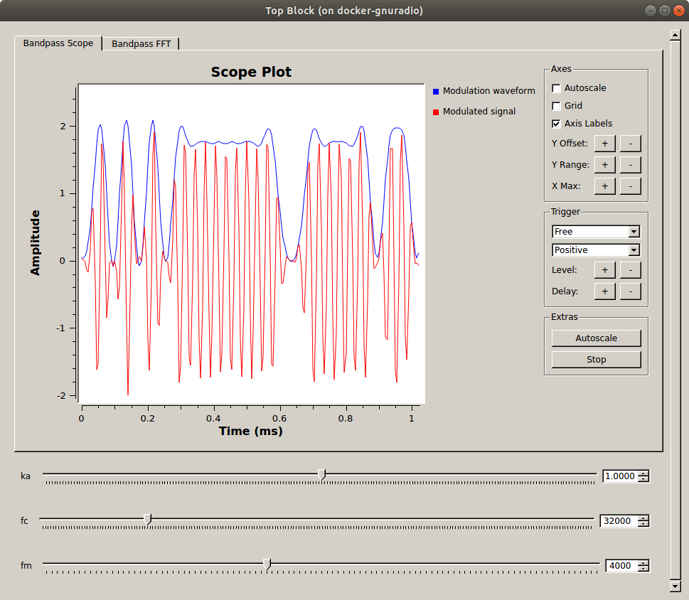
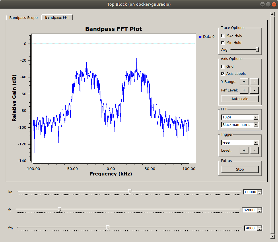
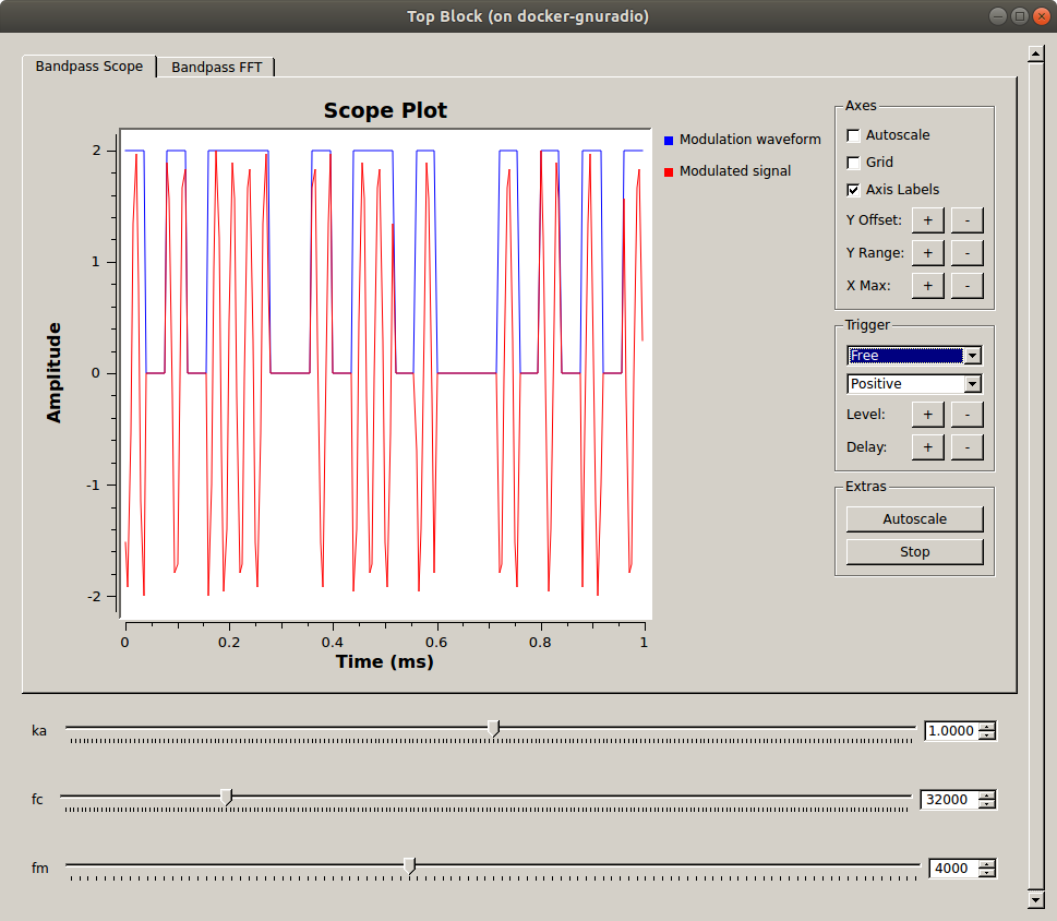
Explore the executed flowgraph. How does changing \(f_c\), \(k_a\), and \(f_m\) change the band pass time signal? How do they change the bandpass spectrum? The following figures show the default values.

Note

When there are two inputs to a GUI Sink, they are plotted as different colors. You can click on their legend entries to hide and show each one.

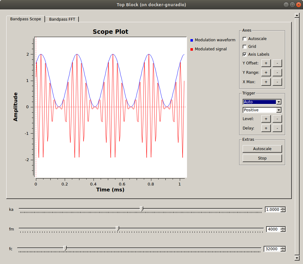
Modulated carrier and modulation waveform

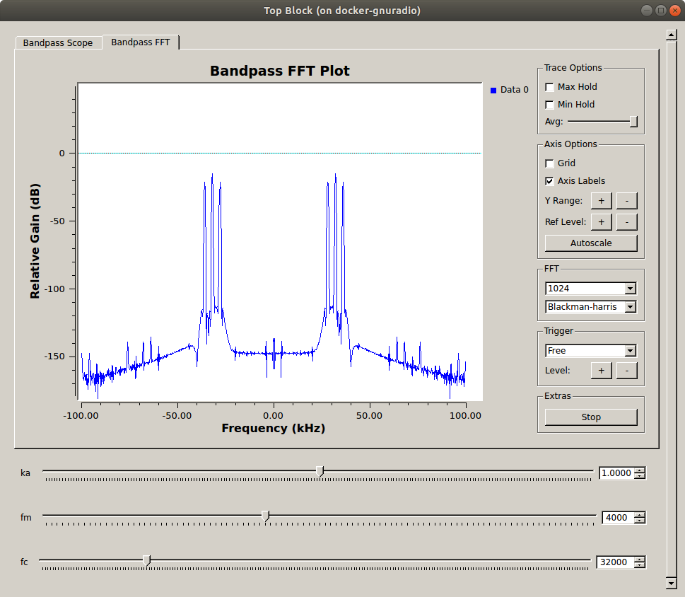
Modulated carrier spectrum

Enable the File Sink, select a save destination and name the output file AM_modulated_4kHz_sine.dat.

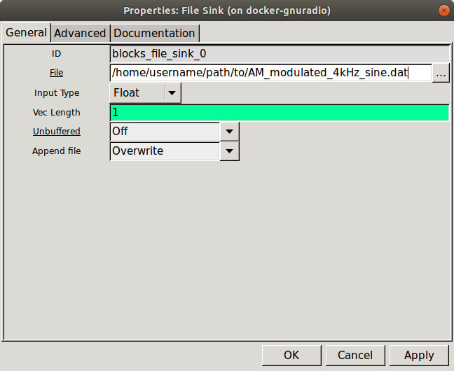
File Sink properties

Execute the flowgraph and after a few seconds kill it. Check that the .dat file now exists by browsing your file systems file explorer. You can now disable the File Sink block again.

Note

If you execute the flowgraph while the File Sink block is enabled, and spend time analyzing the scope and frequency plots, it will be writing to file the entire time. Generally if you want to look at the plots for any duration, you should disable the File Sink block.

A way to regulate the duration a flowgraph runs for is to use the Head block to limit the number of samples that flow either from the input or into the File Sink.

Building an AM transmitter for general messages

Until now, we have only used a sinusoidal message. In this section, we will create four other waveforms and modulate them using amplitude modulation.

Square wave with selectable frequency

Create the following flowgraph to make a symmetric square waveform

Set the sample rate to 200 kHz.
Set a Variable block to have an ID of fm and a value of 4000.
Set the Signal Source block to:
- Waveform: Square
- Frequency: fm
- Amplitude: 2
- Offset: -1
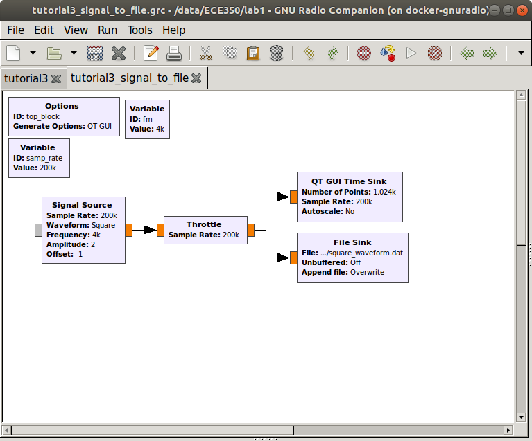
Square waveform generator

This flowgraph will be your second deliverable. Name it waveform_builder.grc, and in the Options block, set the following:

Title: Waveform builder
Author: V00xxxxxx, V00yyyyyy (where all of your student numbers are included)

You can save the generated waveform by re-enabling the File Sink block. Choose a destination to save the file at, and name the file square_waveform.dat.

Go back to your AM Modulator flowgraph and:

change the Signal Source block to a File Source block
- Ensure that you change the correct signal source. You are replacing \(m(t)\) not \(f_c\).
set the source file to square_waveform.dat (the one you just created!)
enable to File Sink block, choose a save destination, and name the file AM_modulated_square.dat
execute the flowgraph.

Modulated carrier and square modulation waveform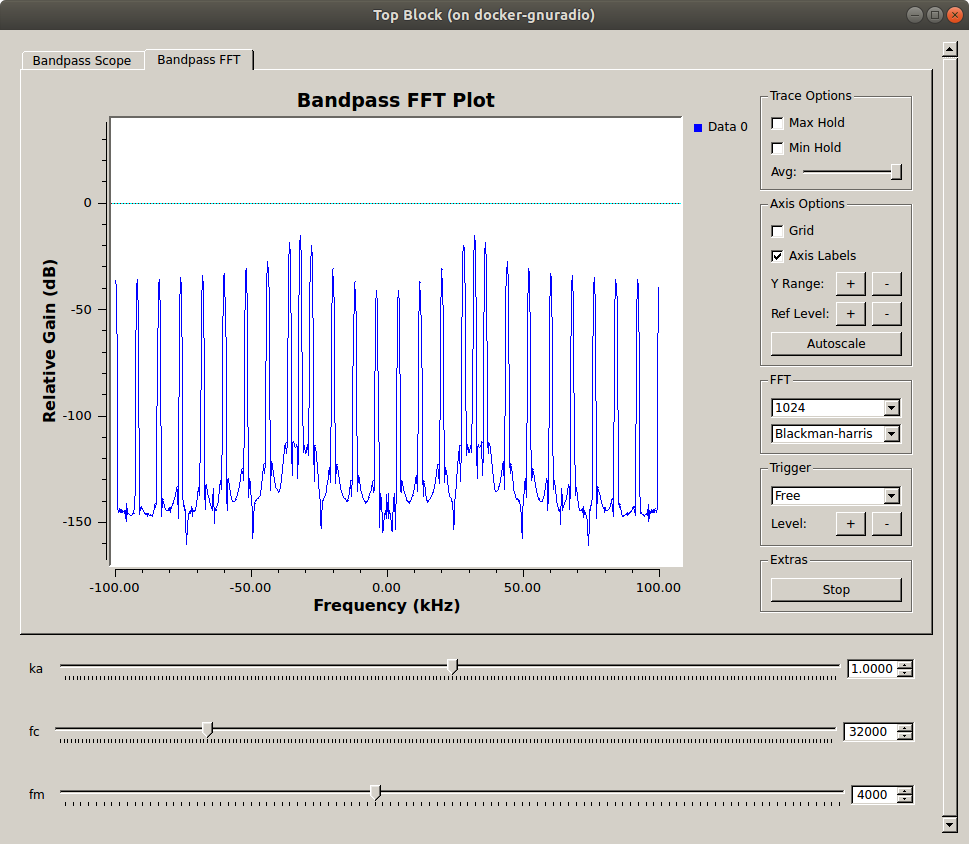

Modulated carrier spectrum for a square AM signal

Two sine waves with selectable frequencies

Update the waveform_builder.grc flowgraph as below, where two sinusoidal signals with frequencies \(f_1\) and \(f_2\) are mixed together to create a two-tone signal with \((f_1-f_2)\) and \((f_1+f_2)\) tones.

Update the Signal Source blocks to use the new variables, f1 and f2.
Ensure the Signal Source block with the square waveform is disabled.
Save the output file as two_sines_waveform.dat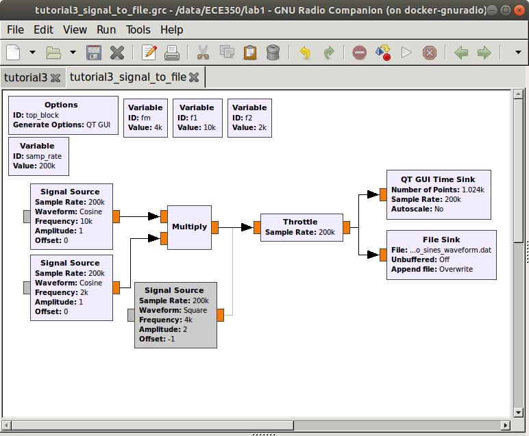

Two sines multiplied and saved to a .dat file

Use the new two_sines_waveform.dat in your AM modulator, saving the output as AM_modulated_two_sines.dat.

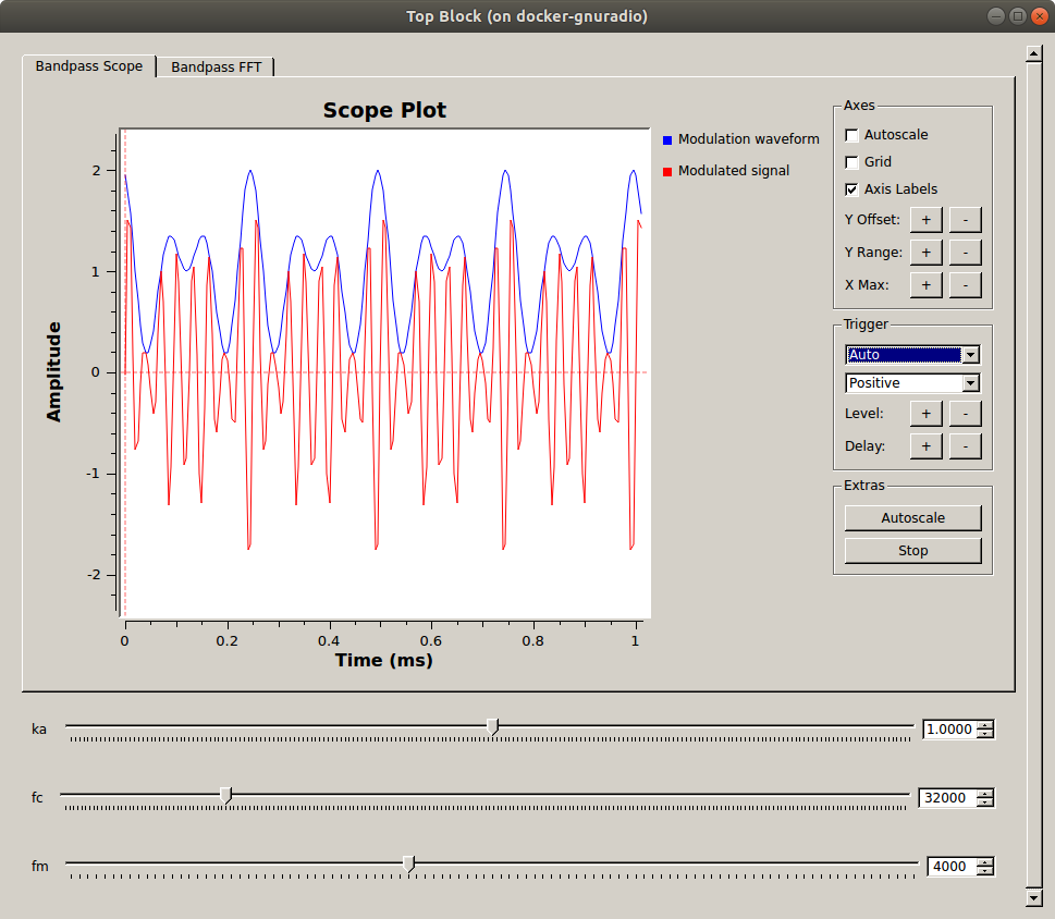
Modulated carrier and two sines modulation waveform

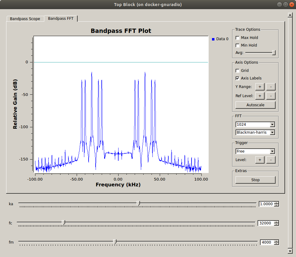
Modulated carrier spectrum for a two sines AM signal

Pseudo Random Binary Sequence (PRBS) with time domain raised cosine pulse shape over 6 symbols

Once again edit the waveform_builder.grc flowgraph to the following. In it, a message signal is created from a sequence of random binary bits which is converted to a sequence of pulses shaped using a raised cosine pulse shaping filter.

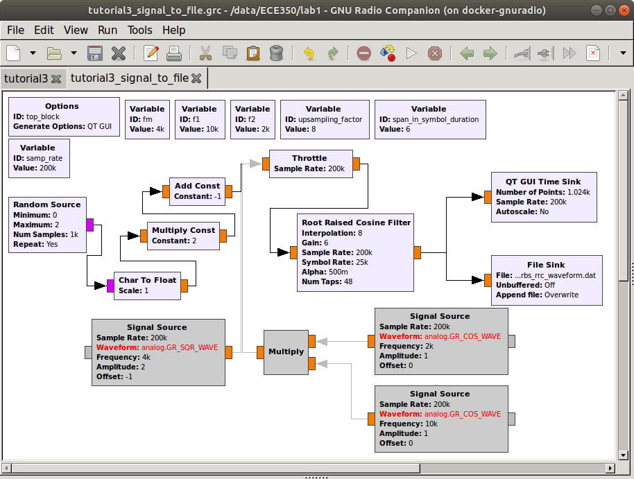
PRBS with a root raised cosine shape saved to a .dat file

The Random Source block generates a sequence of 1000 random bits which is repeated by keeping the Repeat option as “Yes”. The output type is “Byte” which is then converted to “Float” using a Char to Float block. The sequence of {0,1} bits are converted to {-1,1}, which is symmetric about zero by setting the parameters of the Multiply Const and Add Const blocks to 2 and -1 respectively.

The sequence of {-1,1} is converted to a sequence of pulses using the Root Raised Cosine Filter block. The main parameter of a raised cosine filter is it’s roll-off factor (\(\alpha\)), which indirectly specifies the bandwidth of the filter. Ideal raised cosine filters have an infinite number of taps. Practical raised cosine filters are windowed. The window length is controlled here using the span_in_symbol_duration variable. Here, we specify the window length as 6 symbol durations (i.e. the filter spans six symbol durations). Raised cosine filters are used for pulse shaping, where the signal is upsampled. To do this, specify the upsampling factor to match the upsampling_factor variable.

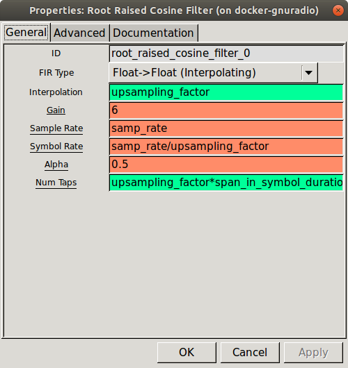
Root Raised Cosine Filter properties

Save the output as prbs_rrc_waveform.dat and run it through the AM modulator, saving the modulator output as AM_modulated_prbs_rrc.dat.

Modulated carrier and PRBC with RRC modulation waveform

Modulated carrier spectrum for a PRBS with RRC AM signal

PRBS with square pulse shape over 6 symbols

Edit the waveform_builder.grc flowgraph and change the Root Raised Cosine Filter block to a Interpolating FIR Filter block, where all 8 of the taps are set to 1. This will make the pulse shape a square.

Note

In some versions of GR the taps need to be contained inside brackets. If you get an error running your interpolation filter set the taps to [1,1,1,1,1,1,1,1] including the brackets.

Note

When a block is yellow in GRC it is in ‘bypass mode’ where the samples pass through the block untouched. This can be done by right-clicking on the block and selecting ‘bypass’ or by pressing ‘b’ on your keyboard.

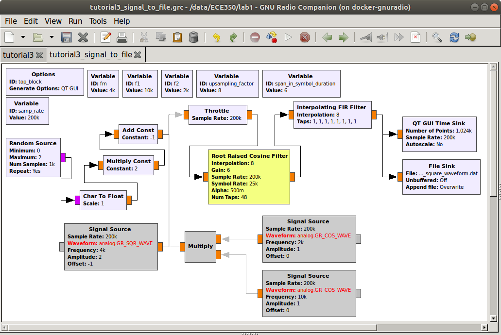
PRBS with a square shape saved to a .dat file

Save the waveform to prbs_square_waveform.dat and run it through the AM modulator. Save the modulated signal as AM_modulated_prbs_square.dat.

Modulated carrier and PRBC with square shape modulation waveform

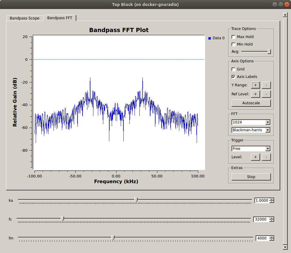
Modulated carrier spectrum for a PRBS with square shape AM signal

Deliverable Question 2

Why are the peaks of the modulated signal (shown above in red) not all the same value (a theoretical value of 2)?

From this section you should have:

two GRC files
- waveform_builder.grc
- AM_modulator.grc
9 data files
- AM_modulated_4kHz_sine.dat
- square_waveform.dat
- AM_modulated_square.dat
- two_sines_waveform.dat
- AM_modulated_two_sines.dat
- prbs_rrc_waveform.dat
- AM_modulated_prbs_rrc.dat
- prbs_square_waveform.dat
- AM_modulated_prbs_square.dat

Review the section deliverables before moving on.

You do not need to attach the top_block.py or .dat files. You will use some of the .dat files in the next part though, so don’t delete them yet!