Part 1 - IQ and using an SDR

Objectives

This part of the lab will guide you through receiving and transmitting signals using a software-defined radio. While using the SDR as a receiver you will learn about:

frequency offsets,
clock sources and reference signal synchronization,
dynamic range and clipping.

While transmitting with the SDR, you will:

see the effect of transmitting real signals, as well as complex signals,
explore the minimum and maximum power output from the SDR,
measure the power of the SDRs transmission using both an oscilloscope and a spectrum analyzer.

Part 1 Deliverables

There are three deliverable questions in this part of the lab. They are clearly indicated.
- Each question requires approximately 1 line of writing and addresses concepts, not details. Answer the questions and submit a single page containing the answers to your TA at the end of the lab.

Be careful

This lab section is possible to do at UVic in the Communications/SDR lab (A309) using an Ettus USRP and also remotely using an RTL-SDR. If you are unsure which to complete talk to your TA. Make sure to pick the right tab below (between USRP and RTL-SDR) so that you don’t complete the wrong lab instructions.

USRP
RTL-SDR

Setup

The small grey box is the USRP software‐defined radio. The USRP digitally downconverts the received (Rx) input signal into I/Q format and sends it via Ethernet to the computer. The USRP also digitally upconverts an I/Q signal from the computer to an RF signal at the transmitter (Tx) output. The USRP’s Rx input is connected to a VHF (Very High Frequency) antenna on the ELW roof. The Tx output can be connected to the oscilloscope and spectrum analyzer.

Verify that the USRP at your station is connected as shown below. If it does not, there are BNC connector cables available at the front of the lab.

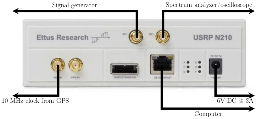
USRP front panel

I/Q Receiver

For detailed information on the usage of the USRP, you can find the data sheet and user manual as well as the range of compatible daughterboards at the Ettus website for the USRP N210.

Refer to the following block diagram to understand the receive path of the USRP as it is set up in the lab. The USRPs in the lab have the WBX daughtercard installed which feature a programmable attenuator, programmable local oscillator and analog I/Q mixer. The WBX daughterboard is an analog front end for the GNU Radio software. It consists of a local oscillator implemented as a wideband frequency synthesizer, thus allowing the USRP to receive signals in the range from 50 MHz to 2.2 GHz. The WBX Daughterboard performs complex downconversion of a 100 MHz slice of spectrum in the 50-2200 MHz range down to -50 to +50 MHz range for processing by the USRP motherboard.

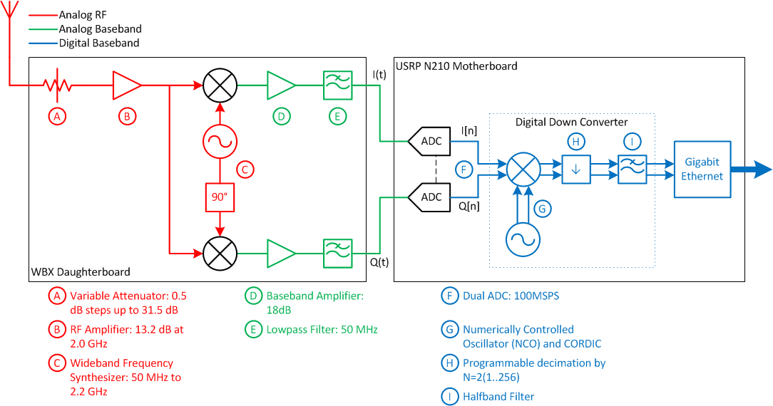
USRP block diagram.

The main function of the USRP motherboard is to act as a Digital Downconverter (DDC). The motherboard implements a digital I/Q mixer, sample rate converter and lowpass filter. The samples are then sent to the host PC over a gigabit ethernet link.

I/Q Receiver output

Review IQ theory in the textbook (Section 1.1).
Download and open the GRC file general-IQ-from-USRP.grc.
- The USRP source does all of the operations in red, green and blue from the figure above. It outputs the complex signal \(I(t) + jQ(t)\).
- This output is connected to 4 blocks that extract the magnitude, phase, real and imaginary parts of the complex signal, as well as a constellation scope.
- The USRP source is tuned to a fixed frequency of 200 MHz, i.e. the LO frequency synthesizer in the WBX daughtercard is set to 200 MHz.
Double‐click the USRP source block to bring up a window with all of the USRP parameters. This general I/Q receiver is set up to receive a signal in a range around 200 MHz at level -10 dBm from the signal generator at the back of the lab.
Execute the flowgraph. Observe the Output Display window with 4 tabs labelled IQ Plane, Magnitude, Phase and IQ Scope Plot.
- The “IQ Plane” tab should show a circle
- The “Magnitude” tab will show a (noisy) DC level
- The “Phase” tab will show a phase ramp wrapping between \(-\pi\) and \(\pi\) (saw-tooth wave) with a period that is the reciprocal of the frequency offset ( \(f_b\))
- The “IQ Scope Plot” tab will show the real and imaginary (noisy) sine waves.
Change the X Max parameter and use the Autoscale button on some of the plots to get a cleaner display.
Determine the frequency \(f_b\) of the sine waves using the Phase display as well as the Real and Imaginary displays by placing your mouse cursor over the scope plot to show the time offset at different points on the waveform as in the figure below.

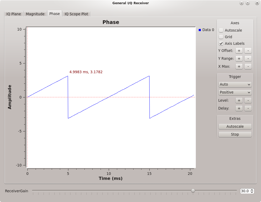
Phase ramp showing frequency offset
This frequency \(f_b\) represents the offset between the received RF signal \(f_c\) and the USRP local oscillator \(f_{LO}\), so that
\[f_b = f_c - f_{LO}\]
The input RF signal is described by:
\[\begin{align*} s(t) &= a(t) e^{j\phi (t)} e^{j2\pi f_c t} \\ &= a(t)cos\left( 2\pi f_c t + \phi (t)\right) + ja(t)sin\left( 2\pi f_c t+ \phi (t) \right) \end{align*}\]
The local oscillator is described by:
\[e^{-j\pi f_{LO} t} = cos\left( 2\pi f_{LO} t \right) - jsin\left( 2\pi f_{LO} t \right)\]
When the two are multiplied, and \(f_b = f_c - f_{LO}\) is substituted:
\[I(t) = a(t)cos\left( 2\pi f_b t + \phi (t) \right)\] \[Q(t) = a(t)sin \left( 2\pi f_b t + \phi (t) \right)\]
This is how you are able to read \(f_b\) directly off of the phase ramp.
- Confirm that \(f_b\) is as expected (ask your TA for \(f_c\))
- To find \(f_c\), ask your TA or go check the signal generator at the back of the lab.
The USRP source block has the Clock Source set to use an External 10 MHz clock reference frequency, and the same external reference is used for the signal generator. Thus the frequency difference between the USRP source block (local oscillator) and signal generator RF frequency will be observed to be exactly as expected from their respective frequency settings.
- If we change the USRP source block to use an Internal clock reference, then expect to observe some frequency error between the signal generator and the USRP frequency settings as they are running from independent oscillators.
- Try changing the USRP clock source to Internal and repeat the frequency measurement of the I and Q outputs. You will see the frequency drifting over time.

Dynamic range with IQ signals

Ask the TA to vary the 200 MHz signal generator level from ‐10 dBm (dB relative to one milliwatt) to 10 dBm in 1 dB steps. Some of the steps are shown in the figures below.
Observe and describe how the signals look at each signal level, and explain why.

The waveform appearance results from clipping in the 2 ADCs (one ADC for I, one ADC for Q).

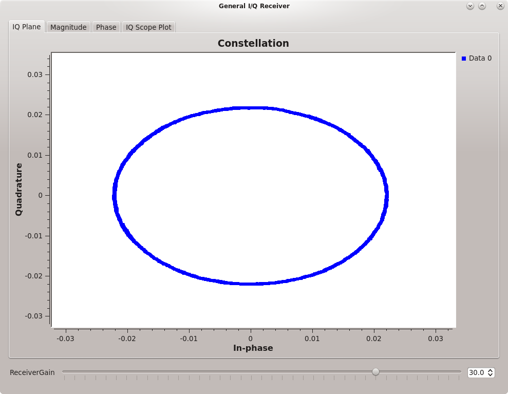
Round constellation plot showing no clipping in the ADCs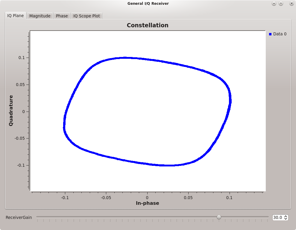

Squashed constellation plot showing some clipping in the ADCs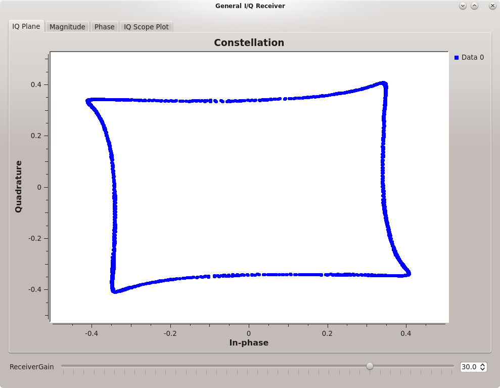

Square constellation plot showing extreme clipping in the ADCs

Deliverable Question 1

Why do you see the constellation plot of the I/Q plane get squashed from a circle into a square as you increase the power of the received signal?

Look at the plot of the phase now. Why does the phase ramp become a staircase? How does this relate to the constellation diagram?

IQ Transmitter

Carrier wave transmission

In this section, we test the transmit functions of the USRP that we can use later when building a communications system. We will observe the transmitted spectrum, minimum and maximum power level in dBm. You will use both the osciloscope and the spectrum analyzer at your bench to view and measure the output from the USRP transmitter.

Review the theory of spectrum analyzers (section 1.4)

For more detailed information, you may also wish to review Spectrum Analyzer Basics and The Basics of Spectrum Analyzers. The concepts presented here will be applicable to any spectrum analyzer you may use in your career.
Download and open this GRC file.
Observe that the USRP sink center frequency is set to 50 MHz. This block represents the USRP transmitter hardware.
Observe that the sine and cosine signal sources are configured for 10 kHz.
Connect the USRP Tx output to the spectrum analyzer and execute the flowgraph. A scope display will come up along with three buttons that allow you to select different values for Q(t).
Set the spectrum analyzer’s center frequency to 50 MHz and the span to 50 kHz by using the FREQUENCY and SPAN buttons. Adjust the LEVEL as necessary.
What do you observe on the spectrum analyzer display with Q(t) = 0? Try the other two options for Q(t). What do you observe on the spectrum analyzer?

Deliverable Question 2

The GRC flowgraph shows a complex stream getting fed into the USRP. How come when Q(t)=0 a real spectrum is shown on the spectrum analyzer?

USRP power levels

What is the minimum and maximum signal power output from the USRP? The USRP output power level can be set via the QT GUI Range Widget seen when running the flowgraph.

Deliverable Question 3

Why, when the USRP is active in transmit-mode, is its minimum output power greater than 0?

Setup

To do this lab remotely you will need an RTL-SDR. It is recommended that you install CubicSDR to test out your radio. It is a user-friendly piece of software which will allow you to find signals and troubleshoot your GNU Radio flowgraphs.

The RTL-SDR digitally downconverts the received (Rx) input signal into I/Q format and sends it via USB to the computer. The RTL-SDR is not capable of transmitting signals.

Plug your RTL-SDR into your computer (remove any connected antenna) and using CubicSDR tune to 144 MHz. You should see an internally generated tone like in the figure below.

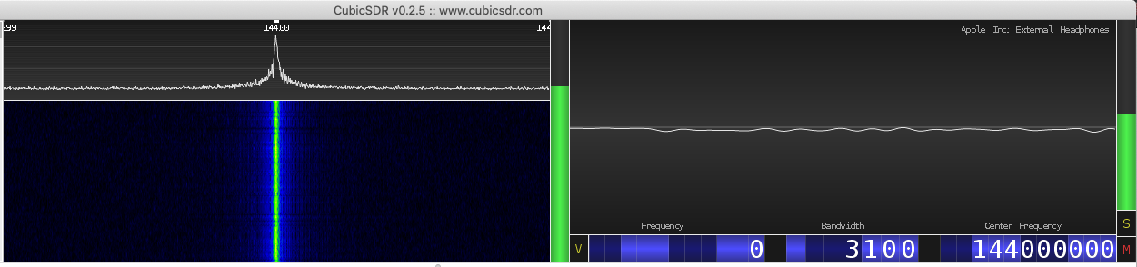
Internally generated 144 MHz tone

I/Q Receiver

For detailed information on the usage of the RTL-SDR, you can find data sheets, user manuals as well as quickstart guides and tutorials at the dedicated RTL-SDR website.

Although the USRPs are not available to you for this lab, it is still useful to review how they work. USRPs are far more powerful than the RTL-SDR and very well documented.

Refer to the following block diagram to understand the receive path of a USRP as they are set up at UVic. The USRPs in the lab have the WBX daughtercard installed which feature a programmable attenuator, programmable local oscillator and analog I/Q mixer. The WBX daughterboard is an analog front end for the GNU Radio software. It consists of a local oscillator implemented as a wideband frequency synthesizer, thus allowing the USRP to receive signals in the range from 50 MHz to 2.2 GHz. The WBX Daughterboard performs complex downconversion of a 100 MHz slice of spectrum in the 50-2200 MHz range down to -50 to +50 MHz range for processing by the USRP motherboard.

USRP block diagram.

RTL-SDR is a name used by a variety of dongles which are all based on the same premise - making cheap SDRs easily available and supported by open-sourced software. Depending on which dongle you have it may be able to receive frequencies from 500 kHz up to 2 GHz.

I/Q Receiver output

Review IQ theory in the textbook (Section 1.1).
Download and open the GRC file general-IQ-from-RTL.grc.
- The RTL-SDR Source block outputs the complex signal \(I(t) + jQ(t)\).
- This output is connected to 4 blocks that extract the magnitude, phase, real and imaginary parts of the complex signal, as well as a constellation scope and waterfall plot.
- The RTL-SDR Source is tuned to a frequency of 144 MHz.

Note

You may need to set the device argument to rtl=0. Try with and without and see what works on your system!

Execute the flowgraph. Observe the waterfall plot and see that there is a signal right in the center of the received spectrum at 144 MHz. Now observe the Output Display window with 4 tabs labelled IQ Plane, Magnitude, Phase and IQ Scope Plot.
- The “IQ Plane” tab should show a circle. Turn up the RF Gain parameter to 60 and see if the increased gain makes the circle bigger. This makes sense as the amplitude of the received signal has become larger.
- The “Magnitude” tab will show a (noisy) DC level
- The “Phase” tab will show a phase ramp wrapping between \(-\pi\) and \(\pi\) (saw-tooth wave) with a period that is the reciprocal of the frequency offset ( \(f_b\))
- The “IQ Scope Plot” tab will show the real and imaginary sine waves.
Change the X Max parameter and use the Autoscale button on some of the plots to get a cleaner display.
Determine the frequency \(f_b\) of the sine waves using the Phase display as well as the Real and Imaginary displays by placing your mouse cursor over the scope plot to show the time offset at different points on the waveform as in the figure below.

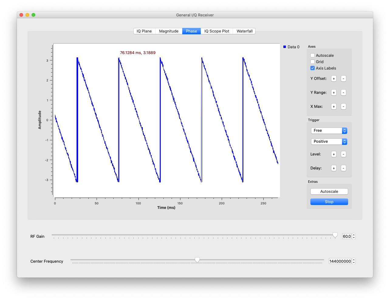
Phase ramp showing frequency offset
As described above, this frequency \(f_b\) represents the offset between the received RF signal \(f_c\) and the SDR’s local oscillator \(f_{LO}\), so that
\[f_b = f_c - f_{LO}\]
The input RF signal is described by:
\[\begin{align*} s(t) &= a(t) e^{j\phi (t)} e^{j2\pi f_c t} \\ &= a(t)\cos\left( 2\pi f_c t + \phi (t)\right) + ja(t)\sin\left( 2\pi f_c t+ \phi (t) \right) \end{align*}\]
The local oscillator is described by:
\[e^{-j\pi f_{LO} t} = \cos\left( 2\pi f_{LO} t \right) - j\sin\left( 2\pi f_{LO} t \right)\]
When the two are multiplied, and \(f_b = f_c - f_{LO}\) is substituted:
\[I(t) = a(t)\cos\left( 2\pi f_b t + \phi (t) \right)\] \[Q(t) = a(t)\sin \left( 2\pi f_b t + \phi (t) \right)\]
Since instantaneous (and in this case unchanging) frequency is the derivative of phase, you can find the slope of the phase plot and that is \(f_b\). Measuring the slope of the phase ramp is how you are able to read \(f_b\) directly from the “Phase” tab of the QT GUI Sink.

Note

Note that there is no ‘amplitude’ on this phase plot - the phase is just wrapping from \(-\pi\to\pi\). When we find the slope we are finding the time it takes for 1 period of \(f_b\) which is the time it takes for 1 ‘wrap’ of the phase ramp. Do not think of finding slope as ‘rise over run’ unless you are aware that the ‘rise’ is 1 period (not 6.28)!

Assuming that \(f_c\) is exactly 144 MHz, use the phase ramp to find your RTL-SDRs local oscillator frequency. Confirm your solution for \(f_{LO}\) with your TA.

Dynamic range with IQ signals

Note

This section is possible to do in practice if you have a signal generator nearby. If so, set it to generate a 200 MHz tone with a small amplitude (when done in the lab the starting amplitude is -10 dBm) and plug the output into your RTL-SDR using a coaxial cable. Then slowly and carefully (so as not to fry your SDR), increase the amplitude until you see what is outlined below.

If using a signal generator to feed this tone into your RTL-SDR note that the maximum allowable input power to the RTL-SDR is 10 dBm.

If you do not have a signal generator at home read along with the following explanation instead.

As your radio receives a pure tone, the constellation looks like the following figure.

Round constellation plot showing no clipping in the ADCs

As the amplitude of the signal is increased, the radius of the circle grows until the ADCs (one for I and one for Q) begin clipping and the constellation starts to get “squashed” as in the following figure.

Squashed constellation plot showing some clipping in the ADCs

This continues until the constellation is a square at which point increasing the signal amplitude makes no difference to the constellation.

Square constellation plot showing extreme clipping in the ADCs

Deliverable Question 1

Why do you see the constellation plot of the I/Q plane get squashed from a circle into a square as you increase the power of the received signal?

IQ Transmitter

Carrier wave transmission

The RTL-SDR is a receive-only SDR and so cannot transmit signals. Follow along with the description and simulation below to explore some key ideas to do with SDR transmission.

Download this GRC file.

Review the theory of spectrum analyzers (section 1.4)

For more detailed information, you may also wish to review Spectrum Analyzer Basics and The Basics of Spectrum Analyzers. The concepts presented here will be applicable to any spectrum analyzer you may use in your career.

Look through the simulation and understand what is happening. Two real signals (\(I(t)\) and \(Q(t)\)) are combined into a single complex signal (\(I(t)+jQ(t)\)). The simulation has been setup so that \(I(t)=\cos \left( 2\pi f_c t \right)\) and \(Q(t)\) is set using the GUI to one of:

\[Q(t)=0\]
\[Q(t)=\sin\left( 2\pi f_c t\right)\]
\[Q(t)=-\sin\left( 2\pi f_c t\right)\]

That makes the complex signal in the three cases:

\[\begin{align*} \tilde{s}(t) =&\sin\left( 2\pi f_c t\right) + 0 \\ =&\Re \{ e^{j2\pi f_c t} \} \end{align*}\]
\[\begin{align*} \tilde{s}(t) =&\sin\left( 2\pi f_c t\right) + j\cos\left( 2\pi f_c t\right) \\ =& e^{j2\pi f_c t} \end{align*}\]
\[\begin{align*} \tilde{s}(t) =&\sin\left( 2\pi f_c t\right) - j\cos\left( 2\pi f_c t\right) \\ =& e^{-j2\pi f_c t} \end{align*}\]

Now consider this exact same setup but where you have an SDR transmitting a complex signal. The complex signal is made up of two tones, a cosine and a sine as in the figure below.

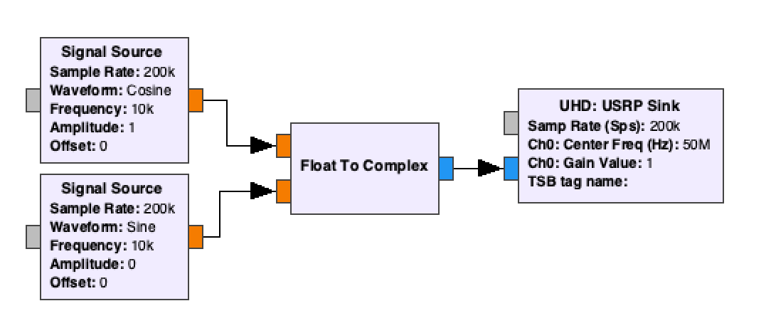
GRC block diagram to transmit a complex signal through a USRP.

Notice that:

the SDR’s center frequency is set to 50 MHz,
the sine and cosine signal sources are set to 10 kHz.

What frequency do you expect the transmitted signal to be at? The SDR will take a baseband input and shift it up to the desired passband center frequency. In this case the transmitted signal exists at 50.01 MHz (50 MHz + 10 kHz).

Plugging a USRP into a spectrum analyzer and running this program yields the following output.

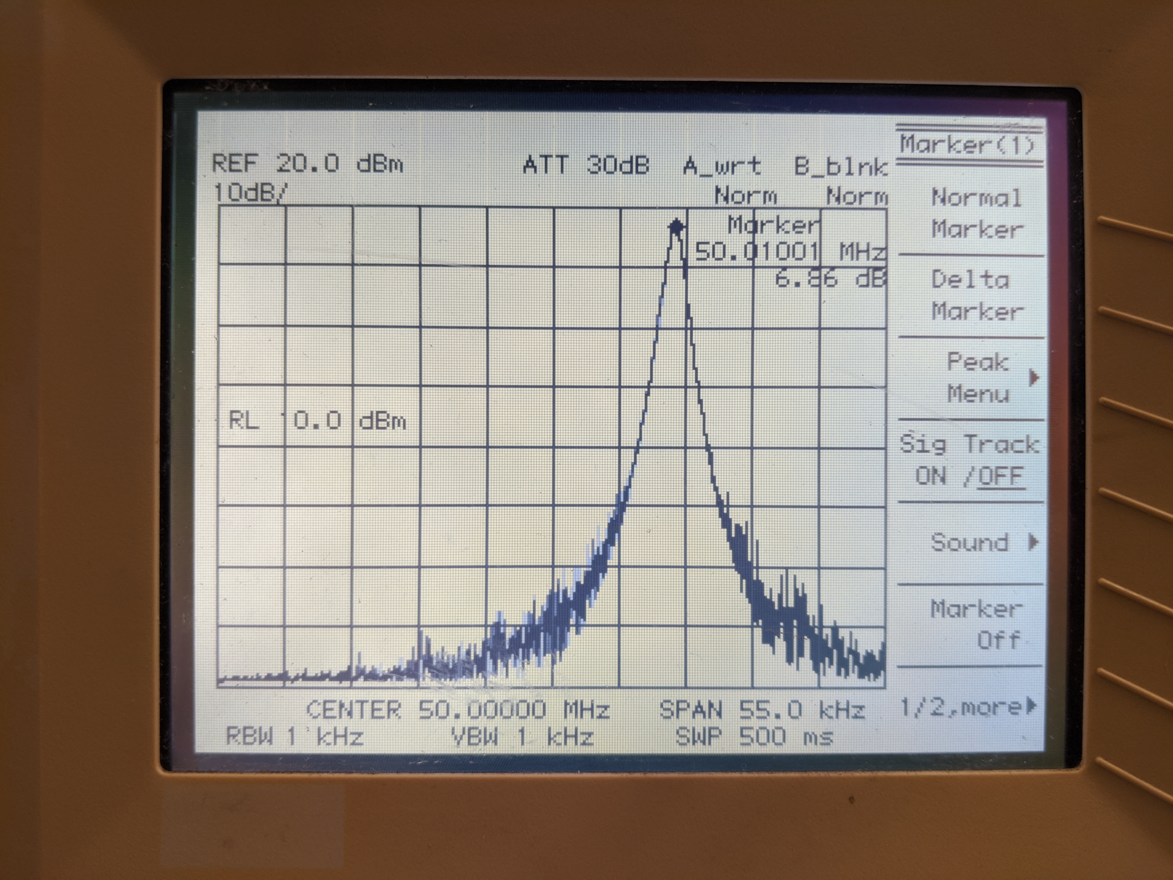
Spectrum analyzer output with \(f_c = 50.01 MHz\).

You can see the same thing by running the above GRC simulation and setting \(Q(t)=sin(2*\pi*f_c*t)\). Look through the simulation to see how this works (what is it changing in the signal source blocks?).

In this case \(f_c = 50.01 MHz\). The signal is complex and can be written as:

\[\begin{align} s(t) &= e^{j2\pi f_c t} \\ &= \cos(2\pi f_c t) + j\sin(2\pi f_c t)\\ \end{align}\]

Now, changing the amplitude of the signal source which makes up \(Q\) to be negative yields the following spectrum.

Spectrum analyzer output with \(f_c = 49.99 MHz\).

Running the simulation and setting \(Q(t)=-sin(2*\pi*f_c*t)\) will show the same thing - a single frequency component shifted down from the center of the spectrum.

In this case the signal can be written as:

\[\begin{align} s(t) &= e^{-j2\pi f_c t} \\ &= cos(2\pi f_c t) - j\sin(2\pi f_c t)\\ \end{align}\]

Finally, changing the amplitude of the signal source which is fed into \(Q\) to be 0 yields the following spectrum.

Spectrum analyzer output with \(f_c = 50 MHz\).

In the simulation, set \(Q(t)=0\) to see this real signal.

In this case the signal can be written as:

\[\begin{align} s(t) &= e^{j2\pi f_c t}+e^{-j2\pi f_c t} \\ &= \cos(2\pi f_c t)\\ \end{align}\]

Deliverable Question 2

The GRC flowgraph simulation shows a complex stream getting fed into the QT GUI Frequency Sink block. How come when \(Q(t)=0\) a real spectrum is shown on the Frequency sink (as well as the actual spectrum analyzer)?

USRP power levels

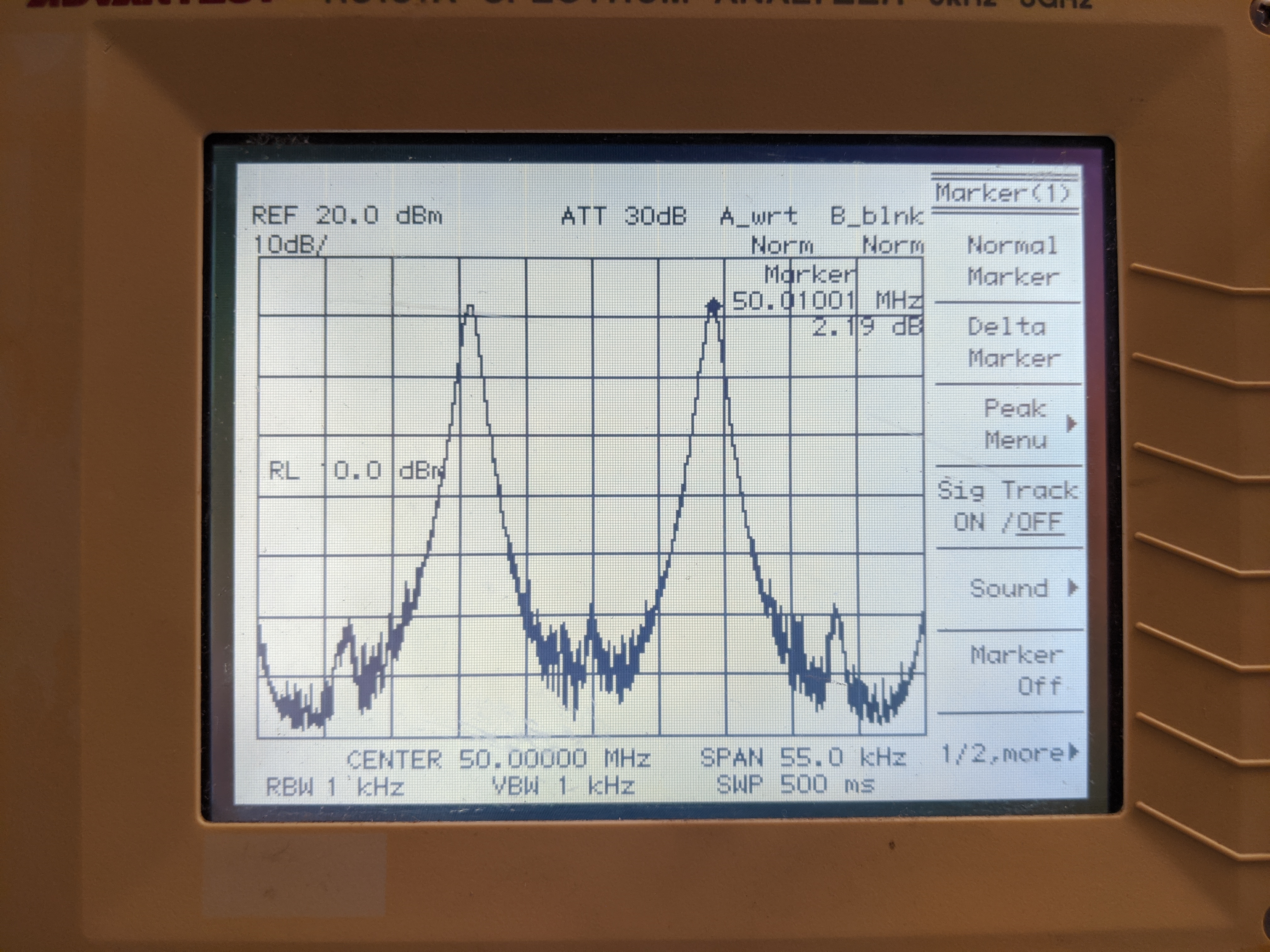
The USRP Sink and RTL-SDR Source blocks include parameters for the radio hardware. In the last section the the radio center frequency was set. Another key parameter is to change the power output by a transmitter. The spectrum analyzer screen shows the following output for a positive gain value (note the dB level of the peak).

Spectrum analyzer output with a positive transmitter gain value.

Without changing the Signal Source blocks, but changing the gain of the transmitter to 0 yields the following spectrum analyzer output. Again note the dB level of the peak.

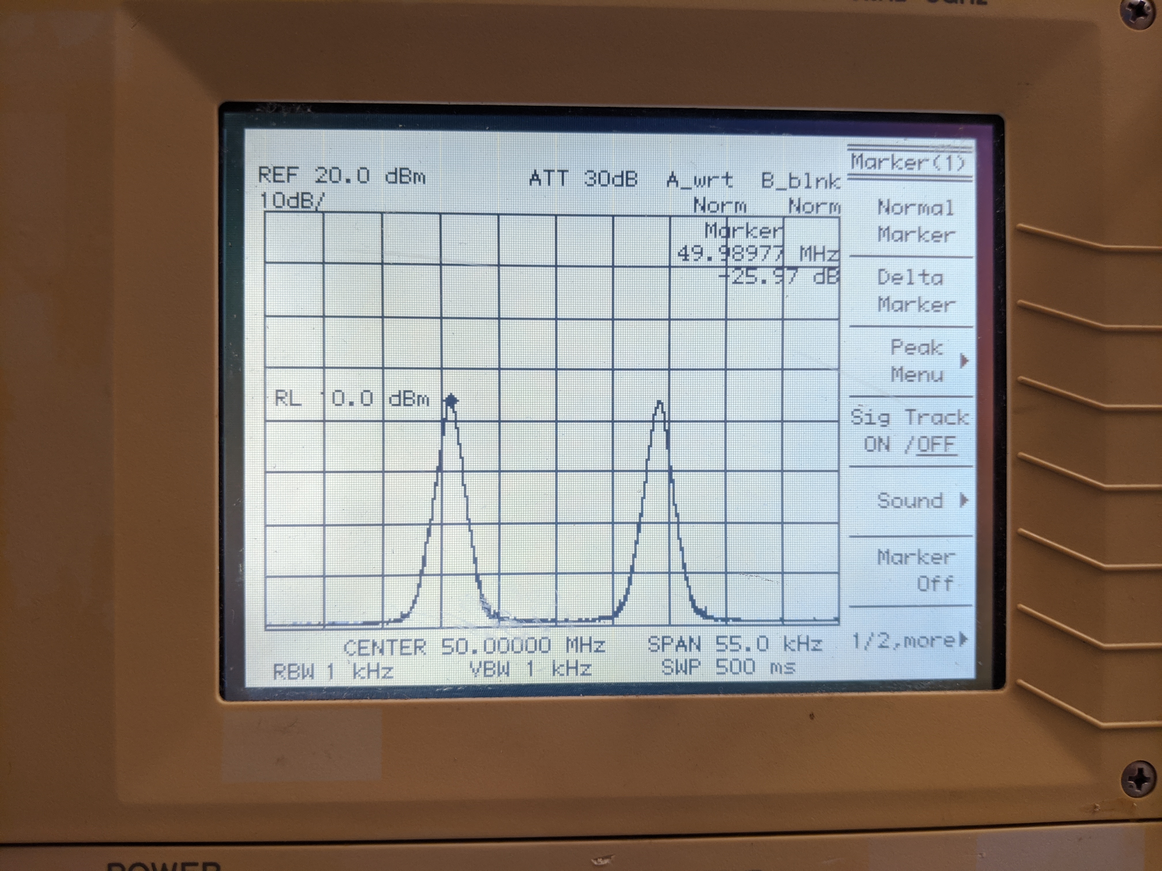
Spectrum analyzer output with a transmitter gain value of 0.

Deliverable Question 3

The USRP is plugged in, powered on and tied with coaxial cable into the spectrum analyzer. Why, when the USRP is active in transmit-mode, is its minimum output power greater than 0?

Deliverables

From this part of the lab keep the following files to submit to your TA:

The answers to 3 deliverable questions.