Part 3 - FM receiver with SDR
Objectives
This part of the lab is a guide to receiving real FM signal waveforms. You will:
- use the previously used delay-conjugate demodulation method to receive real signals and listen to FM radio
- learn the theory of cross-modulation
Part 3 Deliverables
- There are 3 questions in this part. They are clearly indicated.
- Each question requires approximately 1 line of writing, and addresses a concept, not details. Answer the questions and submit a single page containing the answers to your TA at the end of the lab.
- One GRC files of an FM receiver (continued from the last part of the lab).
Be careful
This lab section is possible to do at UVic in the Communications/SDR lab (A309) using an Ettus USRP and also remotely using an RTL-SDR. If you are unsure which to complete talk to your TA. Make sure to pick the right tab below (between USRP and RTL-SDR) so that you don’t complete the wrong lab instructions.
FM broadcast receiver
In this section, we consider a practical FM receiver that can receive real off-air FM signals using the USRP. You will adjust the FM receiver built in the last part of the lab to work with these real signals.
-
Open the FM receiver flowgraph you completed in the last part of this lab.
-
Disable the File Source stream up to and including the Float To Complex block.
-
Enable to USRP Source stream. You will need to reroute the inputs to the Delay and Multiply Const blocks from the newly enabled Low Pass Filter.
Deliverable Question 2
Which blocks from the File Source stream are replaced with the USRP Source block?
Deliverable Question 3
What is the transition width of the low pass filter used on the USRP’s output? Why was this value chosen? (Hint: Consider FM Broadcast channel spacings.)
- Execute the flowgraph and Observe the waterfall and spectrum.
- The radio is tuned to 98.1 MHz (an FM station in Seattle), the RF gain is set to 7.
-
Notice the noise level of the filtered signal is around ‐120 dBm and the signal peak level is 10‐20 dB higher than that.
- This FM receiver is not particularly useful without an audio output.
- Add a Rational Resampler block after the Complex to Arg block and resample the signal to 48 kHz. Set the Type to be Float->Float (Real Taps).
- Add a Multiply Const block with the Constant parameter set to a variable,
af_gain.- Notice that the variable is set using a QT GUI Range block.
- Add an Audio Sink block with the Sample Rate set to 48 kHz.
-
The flowgraph should now look like the following figure.
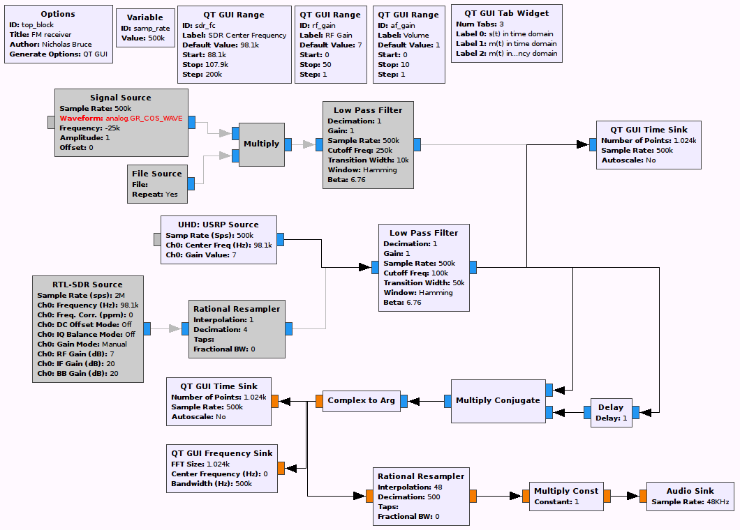
USRP FM receiver with an audio output - Execute the flowgraph. Tune to 101.9 MHz (CFUV) which is the radio station run on UVic’s campus transmitted from the Student Union Building. Sing along.
Dynamic Range with FM
-
Review the theory of dynamic range. These notes will also be useful for subsequent sections on dynamic range with IQ signals and on noise figure.
-
Tune the USRP to the FM broadcast station at 101.5 MHz.
-
Increase the RF gain from 7 dB until you hear a second radio station at the same time, or instead of the original station.
- Notice that the signal level increases and then suddenly both noise and signal jump up and the audio changes to a different program.
What is happening is that a strong signal somewhere within the 40 MHz bandwidth of the USRP’s receiver is clipping the 14 bit A/D converter in the USRP. The 14 bit A/D converter has a dynamic range of about 84 dB (14 bits times 6 dB per bit), so a signal above about ‐100 dBm + 84 dB = ‐16 dBm will clip the converter. With the RF gain set to around 20 dB, the receiver becomes non‐linear and the audio from the strong signal is cross‐modulating on top of the signal at 98.1 MHz.
-
Cross‐modulation can be shown to occur by modelling the non‐linear receiver as having the output:
\[y(t) = a_1 s(t) + a_2 s^2 (t) + a_3 s^3 (t)\](ignoring higher order terms), where \(s(t)\) is the sum of the strong and the weak signal.
-
Reduce the RF gain and notice that the original signal is restored. Next, we will look for this strong signal.
-
Tune the FM receiver to 101.9 MHz (the local UVic radio station CFUV). Notice that the signal level is much higher (close to ‐30 dBm). Now increase the RF gain to at least 20 dB and observe the signal level can be increased to above ‐16 dBm, however, the audio is not changed. This signal at 101.9 MHz was causing the clipping.
-
Experiment more with the FM receiver. Notice that many signals can be received, FM signals are spaced every 0.2 MHz with an odd last digit, from 88.1 MHz up to 107.9 MHz.
FM broadcast receiver
In this section, we consider a practical FM receiver that can receive real off-air FM signals using the RTL-SDR. You will adjust the FM receiver built in the last part of the lab to work with these real signals.
Open the FM receiver flowgraph you completed in the last part of this lab and make the following changes:
- Disable the File Source stream up to and including the streams Low Pass Filter block.
- Enable to RTL-SDR Source stream. You will need to reroute the inputs to the Delay and Multiply Const blocks from the newly enabled Low Pass Filter.
Deliverable Question 2
Which blocks from the File Source stream are replaced with the RTL-SDR Source block?
Deliverable Question 3
What is the transition width of the low pass filter used on the RTL-SDR’s output? Why was this value chosen? (Hint: Consider FM broadcast channel spacings. FM channels exist at the same frequencies everywhere in the world: 88.1 MHz, 88.3 MHz, 88.5 MHz, …, 108.1 MHz. What happens if there are a series of closely packed channels at say 101.1, 101.3 and 101.5 MHz and you want to listen to the station at 101.3 MHz?)
Execute the flowgraph. By default the radio is tuned to 98.1 MHz and the RF gain is set to 7.
- You may find it helpful to add a QT GUI Frequency Sink and/or a QT GUI Waterfall Sink to the output of the RTL-SDR Source block (and set the sampling rate of the sink appropriately). This will allow you to observe where there are FM broadcast stations!
Note
You may need to set the device argument to rtl=0. Try with and without and see what works on your system!
Look up a FM station in your area and tune to it using the slider. When you are centered on it, increase the RF gain until the channel is clearly visible in the spectrum.
Note
Because you are receiving a real-life on-air signal, it will help to have an antenna connected to your RTL-SDR and have the antenna placed near a window.
This FM receiver is not particularly useful without an audio output.
- Add a Rational Resampler block after the Complex to Arg block and resample the signal to 48 kHz. Set the Type to be Float->Float (Real Taps).
- Add a Multiply Const block with the Constant parameter set to a variable,
af_gain.- Notice that the variable is set using a QT GUI Range block.
- Add an Audio Sink block with the Sample Rate set to 48 kHz.
The flowgraph should now look like the following figure.
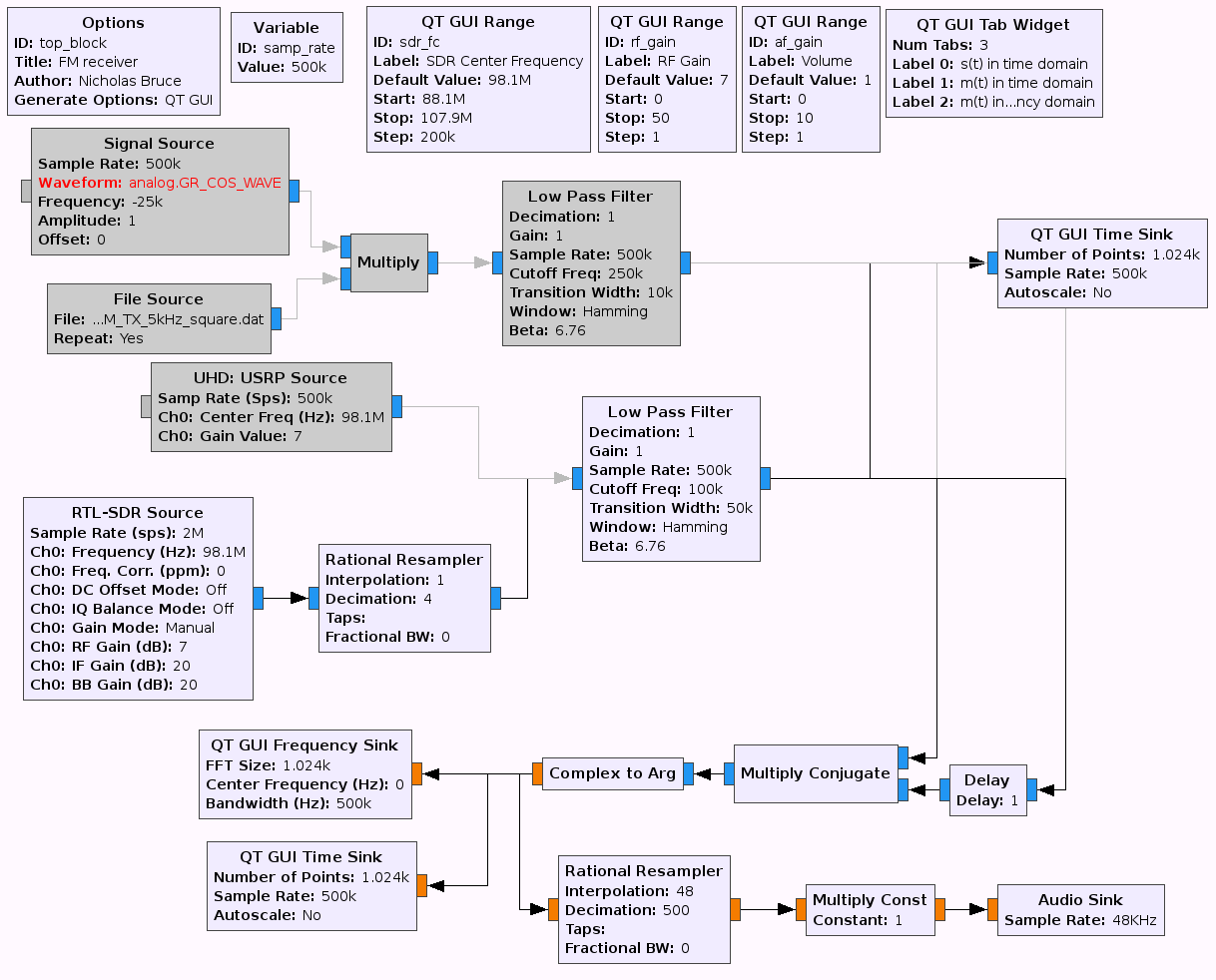
RTL-SDR FM receiver with an audio output
Execute the flowgraph and increase the RF Gain until the audio is legible. Sing along.
Dynamic Range with FM
Review the theory of dynamic range. These notes will also be useful for subsequent sections on dynamic range with IQ signals and on noise figure.
Tune the RTL-SDR to a weak FM channel. You can add a QT GUI Waterfall at the output of the RTL-SDR Source to help search for a weak channel.
Increase the RF gain from 7 dB until you hear a second radio station at the same time, or instead of the original station.
Notice that the signal level increases and then suddenly both noise and signal jump up and the audio changes to a different program. What is happening is that a strong signal somewhere within the 2.4 MHz bandwidth of the RTL-SDR’s receiver is clipping the 8 bit A/D converter in the RTL-SDR. The 8 bit A/D converter has a dynamic range of about 48 dB (8 bits times 6 dB per bit), so a signal 48 dB above the noise floors value will clip the converter.
Cross‐modulation (where a strong signal transfers it’s modulation to a frequency (CW tone) at the receiver input) can be shown to occur by modelling the non‐linear receiver as having the output:
\[y(t) = a_1 s(t) + a_2 s^2 (t) + a_3 s^3 (t)\](ignoring higher order terms), where \(s(t)\) is the sum of the strong and the weak signal.
Reduce the RF gain and notice that the original signal is restored. Next, we will look for this strong signal.
Tune the FM receiver to the strongest FM station you can find. Notice that the signal level is much higher. Now increase the RF gain to at least 20 dB and observe the signal level can be increased to above the previous limit without the audio changing. This signal may have been causing the clipping.
Experiment more with the FM receiver. Notice that many signals can be received, FM signals are spaced every 0.2 MHz with an odd last digit, from 88.1 MHz up to 107.9 MHz.
Deliverables
From this lab part, there are the following deliverables:
-
The answers to two deliverable questions.
-
one GRC file
FM_receiver.grc
Do not attach the top_block.py or .dat files.
UVic ECE Communications Labs
Lab manuals for ECE 350 and 450