Part 2 - FM receiver simulator

Edit me

Objectives

This part of the lab is a guide to receiving FM signal waveforms. You will:

learn the theory and equations of FM signals, power spectra, bandwidths, and FM demodulation
construct an FM receiver flowgraph to recover messages from an FM waveform

Part 2 Deliverables

One GRC files of an FM receiver. You will be stepped through building it.

Theory

Review the theory of FM Signals (section 5).
Recall that a digital FM demodulator starts with the I and Q outputs of a general IQ receiver. For an FM signal,
\[s(t) = A_c cos \left( 2\pi f_c t + 2\pi k_f \int_{0}^{1} m(\alpha )d\alpha \right)\] \[I(t) = A_c cos \left( 2\pi k_f \int_{0}^{1} m(\alpha )d\alpha \right)\] \[Q(t) = A_c sin \left( 2\pi k_f \int_{0}^{1} m(\alpha )d\alpha \right)\]
To extract \(m(t)\) from \(I(t)\) and \(Q(t)\), consider them as a complex signal.
\[\begin{align*} s(t) &= Re \{ a(t) e^{j\phi (t)} e^{j2\pi f_c t} \} \\ &= Re \{ [ I(t) + j Q(t) ] e^{j2\pi f_c t}\} \\ &= Re \{ \tilde{s}(t) e^{j2\pi f_c t } \} \end{align*}\]
where,
\[\begin{align*} \tilde{s}(t) &= I(t) + jQ(t) \\ &= a(t) e^{j\phi (t) } \end{align*}\]
It can be shown that \(m(t)\) is obtained from the following formula:
\[m(t) = arg[ \tilde{s}(t-1) \tilde{s}^{*} (t) ]\]
where,
\[(t-1) \rightarrow z^{-1}\]
represents one sample delay.

Proof: \(\\ \begin{align*} arg[ \tilde{s}(t-1)\tilde{s}^{*} (t) ] &= arg[ a(t-1) e^{j\phi (t-1)} a(t)e^{-j\phi (t)} ] \\ &= \phi (t-1)- \phi (t) \\ &\approx \frac{d\phi}{dt} \\ &\approx 2\pi k_f m(t) \end{align*}\)

Receiving and demodulating simulated FM signals

To begin, download this partially completed flowgraph.
- The completed portion implements three sources:
  - a RTL-SDR Source and filter which are disabled,
  - a USRP Source and filter which are disabled,
  - a File Source, down conversion, and filter which are enabled.
- Each of these sources can be used and controlled with the same QT GUI Range parameters.
- If you want to use the USRP or RTL-SDR as a source, disable the stream coming from the File Source. If you want to use the File Source stream, do the opposite.
- For now, leave the SDR streams disabled and the File Source stream enabled.

The output of each stream is \(\tilde{s}(t)\). Note that the Signal Source used to shift the received signal down by the carrier frequency is set negative 25 kHz.

Open the File Source block and point it at FM_TX_5kHz_sine.dat. Execute the flowgraph and check that the output at \(\tilde{s}(t)\) is as expected (what you saw in the previous section before writing it to this file).
Implement \(m(t) = arg[ \tilde{s}(t-1) \tilde{s}^{*} (t) ]\) from the theory section to extract the message from the baseband signal.
- You will need a Delay block with the Delay property set to 1. This delays every sample that enters the block by 1 sample.
- You will also need one of each a Multiply Conjugate block and a Complex to Arg block.
- Try to do this without looking at the figure of the final flowgraph below. Interpret the math and implement it by using the mentioned blocks.
Add a QT GUI Time Sink and a QT GUI Frequency Sink to the output to view the demodulated message.
- Set the GUI Hint parameter of the time sink to tabs@1.
- Set the GUI Hint parameter of the frequency sink to tabs@2.
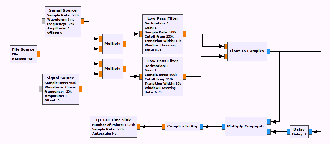
The flowgraph should now look like the following figure.

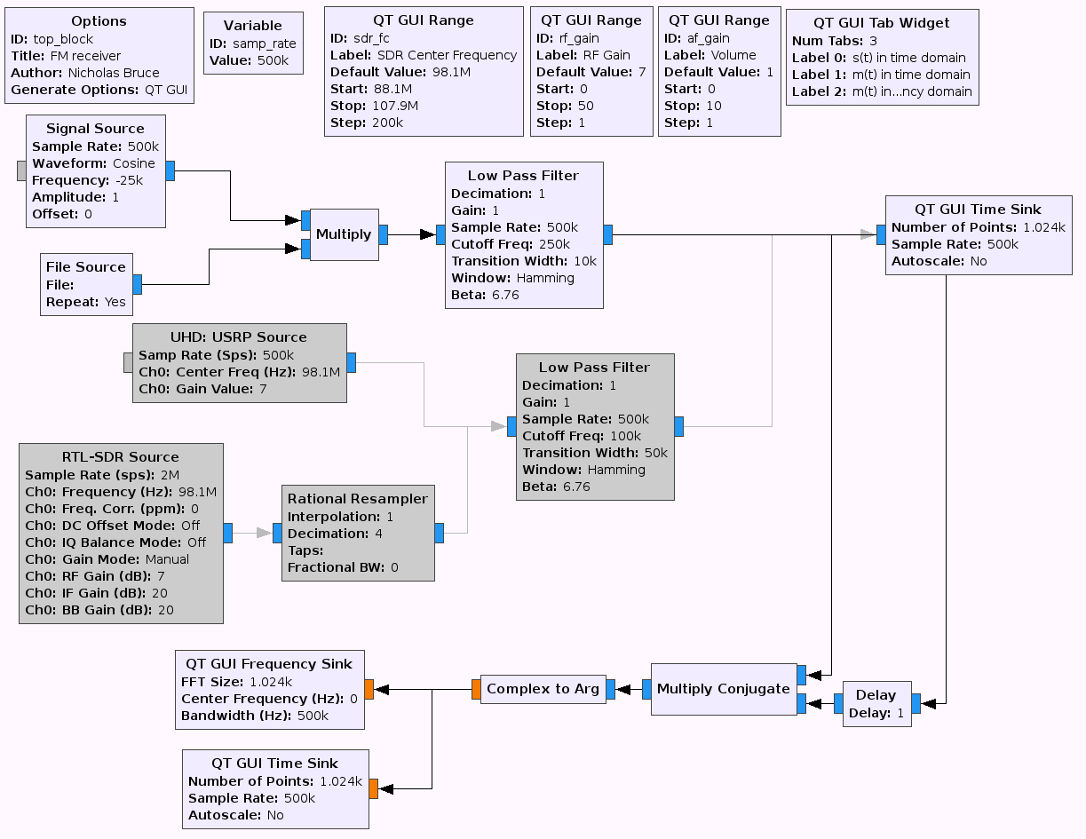
FM receiver flowgraph
Execute the flowgraph. You should see the demodulated 5 kHz sine wave in the output spectrum and time scope.

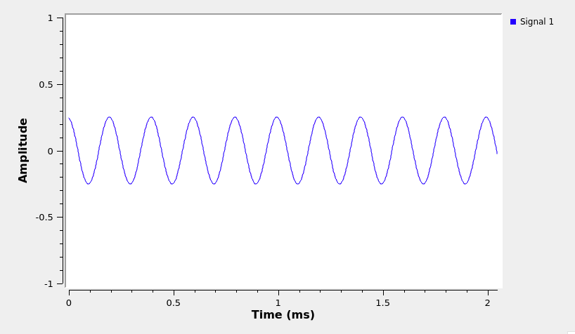
Demodulated sine message, \(m(t)\) in time domain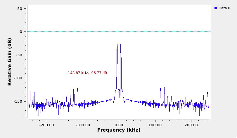

Demodulated sine message, \(m(t)\) in frequency domain
Switch the input file to be FM_TX_5kHz_square.dat. You should be able to read the 1010... FSK sequence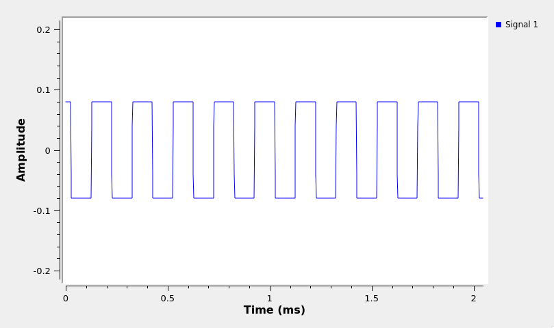

Demodulated FSK message, \(m(t)\) in time domain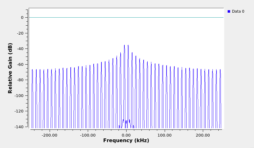

Demodulated FSK message, \(m(t)\) in frequency domain
This flowgraph will be a deliverable. Save it as FM_receiver.grc, and in the Options block, set the following:
- Title: FM receiver
- Author: V00xxxxxx, V00yyyyyy (where all of your student numbers are included)

Advantage of a complex receiver versus a real receiver

The receiver implemented above uses a complex signal for input. A real signal could be used instead but the flowgraph becomes much more complicated. The below flowgraph is equivalent to the one you implemented above.

Real FM receiver which is far more complicated than the complex receiver.

At this point, you should have:

one GRC file
- FM_receiver.grc

Deliverables

From this lab part, keep the following for later submission to your TA:

FM_receiver.grc

You will build upon this flowgraph further in the next part of the lab.

Do not attach the top_block.py or .dat files.