Part 1 - FM transmitter simulation
Objectives
This part of the lab is a guide to transmitting FM signal waveforms. You will:
-
learn the theory and equations of FM signals, power spectra, bandwidths, and FM modulation
-
construct an FM transmitter flowgraph to generate an FM waveform with both a sinusoidal message and a square wave message
Part 1 Deliverables
- One GRC file of an FM transmitter. You will be stepped through building it.
- There is 1 question in this part. It is clearly indicated.
- The question requires approximately 1 line of writing, and addresses a concept, not details. Answer the question and submit a single page containing the answers to your TA at the end of the lab.
You are going to build flowgraphs to transmit FM signals that are simulation-only and do not (yet) use the SDR (that will come later in this lab!).
Theory
- Review the theory of FM Signals (section 5).
-
Recall that for a sinusoidal modulating wave,
\[m(t) = A_{m}cos\left( 2\pi f_m t\right)\]the FM wave can be written as:
\[\begin{align*} s(t) &= A_{c}cos\left( 2\pi f_c t + \beta sin \left(2\pi f_m t \right) \right) \\ &= Re \{ A_c e^{j(2\pi f_c t + \beta sin(2\pi f_m t))} \} \\ &= Re \{ A_c e^{j\beta sin(2\pi f_m t)} e^{j2\pi f_c t} \} \\ &= Re \{ \tilde{s}(t) e^{j2\pi f_c t} \} \\ &= Re \{ s^{+}(t) \} \\ \end{align*}\]
Exploring the Phase Mod block
How do you transmit a real signal (we’ll call it \(\phi\)) as complex (\(e^{j\phi}\)) in GNU Radio? Let’s explore.
-
Open a new GNU Radio Companion flowgraph.
- Add a QT GUI Range block and set its parameters as follows:
- ID:
phi - Default Value: 0
- Start: -3.14
- Stop: 3.14
- Step: 0.01
- ID:
-
Add a Constant Source block and set it’s Constant to be
phi, the variable from the QT GUI Range block. Make sure that the block type is Float. -
Add a Throttle block of type Float
-
Add a QT GUI Constellation Sink and notice that it can only accept complex numbers!
-
Your flowgraph should look like the following figure. The output of the float line is a signal, \(\phi\), and we need the input of the IQ plane to be \(e^{j\phi}\).
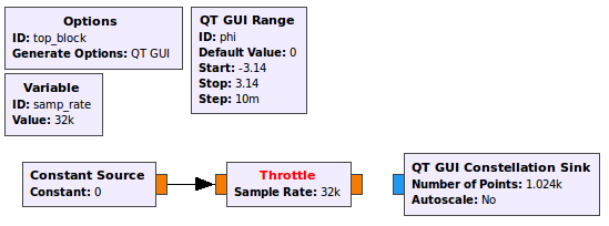
Flowgraph of a real signal unable to be connected to a complex sink - Add a Phase Mod block.
-
Read the documentation on the block to understand what it is doing. It can be described by
\[\textrm{output}=e^{j(\textrm{input})(\textrm{sensitivity})}\] -
Notice the sensitivity parameter. Set it to be 1.
-
-
The input of the Phase Mod block is some GUI controlled number between \(-\pi\) and \(\pi\). The Phase Mod block output is then \(e^{jx\pi}\) where \(x\) is the sensitivity parameter. Notice the \(j\) in the above equation, and also notice the way in which the sensitivity parameter can be used.
-
The flowgraph should now look like the following figure.
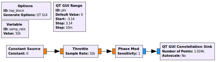
Flowgraph of a real signal being transmitted as a complex signal - Execute the flowgraph. You should see a small dot hovering around \(I = 1, Q = 0\) which is \(e^{j\phi}\) where \(\phi = 0\).
-
As you move the slider from \(-\pi \rightarrow \pi\), you are changing \(\phi\) from \(-\pi \rightarrow \pi\).
- You may discard this flowgraph, it is not a deliverable. However, remember how the Phase Mod block works. You will need to use it later.
Building an FM transmitter for a sine message
You’ll start by transmitting a sinusoidal message. The equations for this are shown in the theory section above.
-
Start GRC and change the default sampling rate to be 500 kHz.
-
This flowgraph will be your first deliverable. Save it as
FM_transmitter.grc, and in the Options block, set the following:- Title: FM transmitter
- Author: V00xxxxxx, V00yyyyyy (where all of your student numbers are included)
- From the equations above, create some variables controlled with sliders.
- Add a QT GUI Range for each of \(f_m\), \(f_c\) and \(\beta\).
- For the message frequency, range from 0-10 kHz with a default value of 5 kHz.
- For the carrier frequency, range from 0-100 kHz with a default value of 25 kHz.
- For the beta value, range from 0-10 with a default value of 4, and a step size of 0.025.
- Begin by using a Signal Source block and a Multiply Const block to create the \(\beta sin( 2\pi f_m t)\) term.
- Use the Multiply Const block for \(\beta\) instead of the Amplitude parameter of the signal source.
- In the signal source, change the Output Type to Float, and the Waveform to Sine.
- Use the variables from the QT GUI Range widgets for \(\beta\) and \(f_m\).
-
This flowgraph will not be used to transmit to any hardware, so a Throttle block is needed. Add a Throttle after the Multiply Const block.
- In order to turn this signal into a complex exponential, we must take \(e^{j\phi}\) where \(\phi\) is the signal at this point.
- Use the Phase Mod block as you did earlier in this lab.
- Notice that we could set the sensitivity parameter to \(\beta\) instead of using the Multiply Const block - the resulting equation is the same!
- Set the Sensitivity parameter to 1.
-
The flow graph should now look like the following figure.
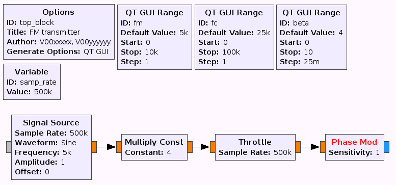
Graphical representation of \(e^{j\beta sin(2\pi f_m t)}\) - Now construct the second exponential, \(e^{j2\pi f_c t}\) and multiply them together to create \(s^{+}(t)\).
- Use a Signal Source block in conjunction with a Multiply block and incorporate the QT GUI Range variable for \(f_c\).
- Use a Complex To Real block to obtain \(s(t)\).
Notice that \(A_c\) is not used and so is equal to 1.
- Visualize the output of the flowgraph using a:
- QT GUI Time Sink at \(m(t)\)
- QT GUI Time Sink at \(s(t)\)
- QT GUI Frequency Sink at \(s(t)\)
As always, you are free to use the QT GUI Tab Widget to organize the GUI however you like. If you need a refresher on how to use this tool, it is covererd in the intro tutorials.
-
The flowgraph should now look like the following figure
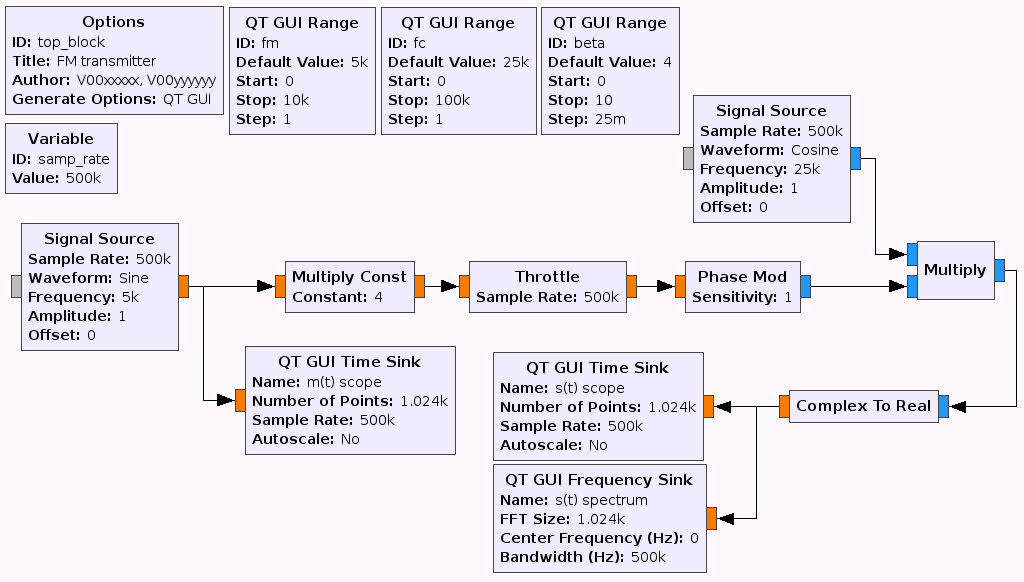
Flowgraph of a FM transmitted sine message -
Leaving default values unchanged, the output should look like the following figures.
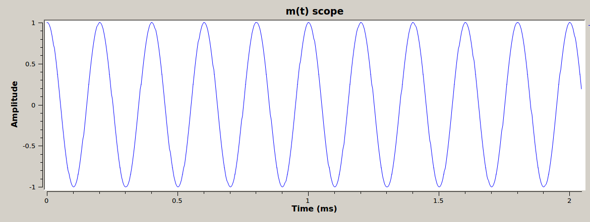
\(m(t)\) with default values in time domain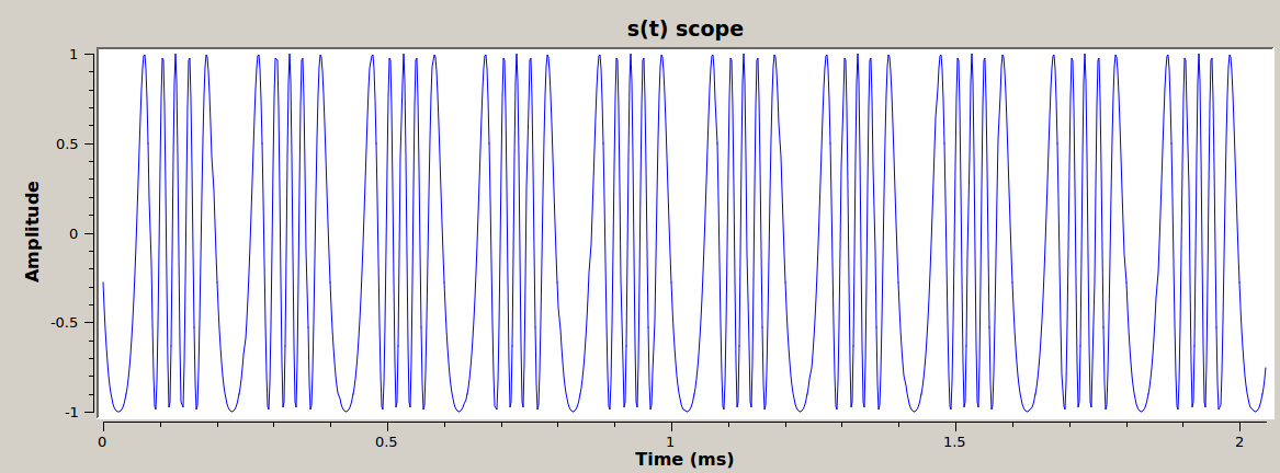
\(s(t)\) with default values in time domain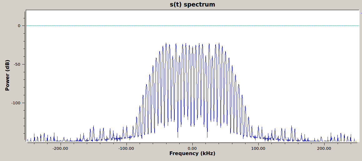
\(s(t)\) with default values in frequency domain -
Experiment with adjusting the three sliders.
-
Reset \(f_c\) to 25 kHz and \(f_m\) to 5 kHz.
- Measure the amplitude of the carrier wave and of the first sideband. To do this zoom in on either the positive or the negative half of the spectrum. Think about what \(f_c\) is set to and find that. The first sideband is the one nearest to it.
The sidebands exist at discrete frequencies of \(\pm f_c \pm n f_m\). Does the spectrum look like this? What are the sidebands spaced by? As you change the \(f_m\) slider do they move? What about if you change the \(f_c\) slider?
Deliverable Question 1
Show that the Bessel peaks have the correct values relative to each other. In other words, confirm that for the chosen value of \(\beta\), the carrier wave and first sideband have the correct values relative to each other as described by the following equation:
\[\Delta P = 20 log\frac{J_1(\beta)}{J_0(\beta)}\]You will want to reference a table of Bessel functions or use a Bessel calculator (built into Matlab/Python/most mathematical programming languages).
- Add a File Sink block to capture the complex output of the Multiply block and save a file called
FM_TX_5kHz_sine.dat. You will need to execute the flowgraph for a few seconds to build the file.
Building an FM transmitter for an FSK message
Up until now the transmitted message has been a sine wave of frequency \(f_m\). You will now simulate transmitting a Frequency Shift Keying (FSK) signal by transmitting a square waveform (which is an FSK pattern of 101010...).
The integral of a square waveform is a triangular waveform with the same frequency as the square waveform. So for frequency modulation with a square wave, we can skip doing the integral and simply use a triangular waveform.
-
Change the Signal Source block to output a triangular waveform of frequency \(f_m\).
-
With the File Sink block disabled, execute the flowgraph and observe the various plots. Adjust the sliders so that \(f_m\) is 2 kHz see how it impacts the transmitted signal. Now change it to 8 kHz.
-
The following figures show \(m(t)\) and \(s(t)\) with a message frequency of 8 kHz.
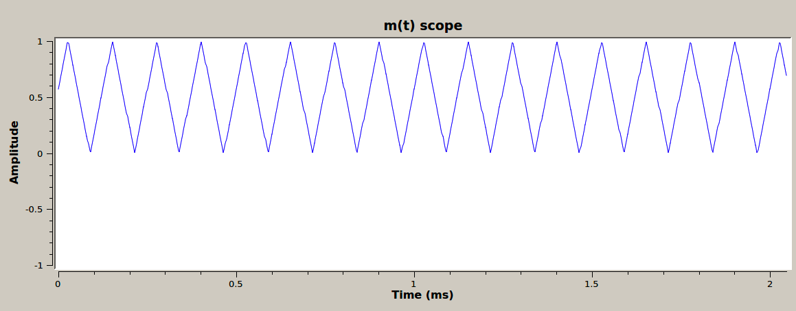
\(m(t)\) with default values in time domain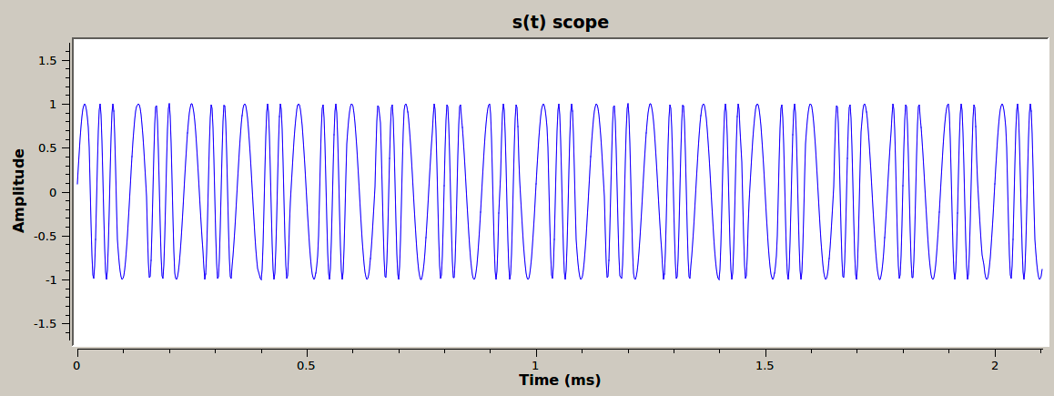
\(s(t)\) with default values in time domain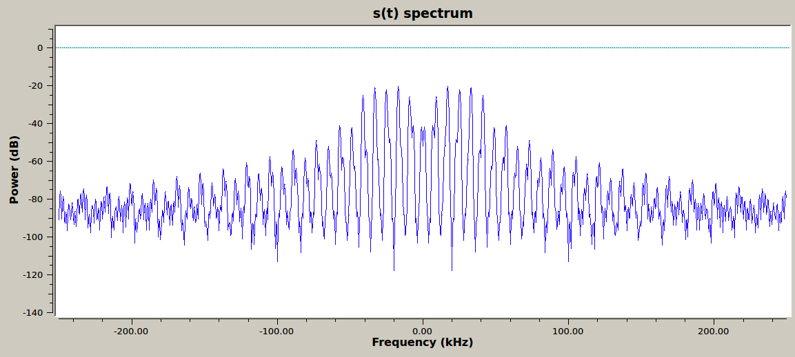
\(s(t)\) with default values in frequency domain
Note
The sidebands for FSK with a square wave message (101010...) do not follow the Bessel function values as they do for a sine wave message.
-
Set the sliders back to default values.
-
Enable the File Sink block and save a file called
FM_TX_5kHz_square.dat. You will need to execute the flowgraph for a few seconds to build the file. -
Save this GRC file now, it is a deliverable.
At this point, you should have:
- one GRC file
FM_transmitter.grc
- 2 data files
FM_TX_5kHz_sine.datFM_TX_5kHz_square.dat
Deliverables
From this lab part, keep the following for later submission to your TA:
FM_transmitter.grc- The answer to one deliverable question.
Do not attach the top_block.py or .dat files. You will use some of the .dat files in the next part though, so don’t delete them yet!
UVic ECE Communications Labs
Lab manuals for ECE 350 and 450