Part 4 - Calculating BER

Objectives

You will use the values recorded to plot a \(BER-\frac{E_b}{N_0}\) curve for each pulse shape and then compare it with theory.

Part 5 deliverables

For this section, the deliverables are:

the answer to three deliverable questions,
the code used to generate the BER curve (with the dataset hard coded into it),
the resulting BER curve as a .PNG image file.

Generating a BER curve

Using the values collected throughout this lab you can now generate a \(BER-\frac{E_b}{N_0}\) curve.

You can use a programming language of your choice, but python or matlab have some handy tools for this job built in.

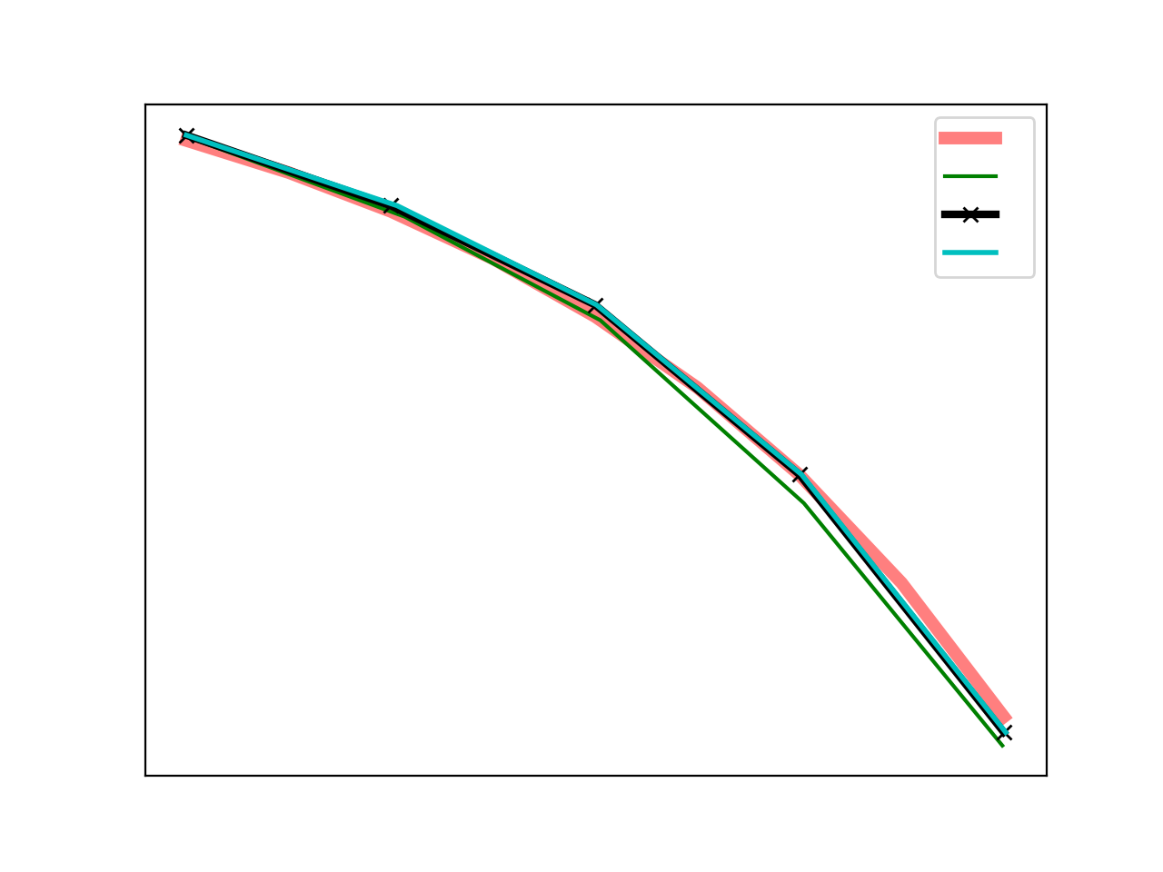
Plot four curves on the same axes:

BER curve for the theoretical \(BER=\sqrt{2\frac{E_b}{N_0}}\),
BER curve using the collected BER values and calculated Eb/N0 values (using the output signal and noise powers) for the LPF flowgraph,
BER curve using the collected BER and Eb/N0 values for the matched filter flowgraph,
BER curve using the collected BER values and calculated Eb/N0 using the collected signal and noise powers at the output of the matched filter.

1. Theory curve

For generating a simulated curve of the theoretical \(BER-\frac{E_b}{N_0}\) review the theory section of this lab. For the Q-function, Matlab ships with qfunc() while python has norm.sf() included in the scipy package.

2. LPF curve

Remember back to the derivation for \(\sigma\) done previously in this lab,

\[\frac{E_b}{N_0}=\frac{1}{2}\frac{a_{out}^2}{\sigma_{out}^2}, \text{(all in linear terms)}\]

Use the signal power and noise powers measured at the output of the matched filter to calculate Eb/N0 values to match the collected BER values.

The BER values collected from the number sink are log10(BER). So to obtain the BER you will need to raise your collected values, -X by realizing that \(BER = 10^{-X}\).

3. RRC curve with user-set Eb/N0 values

You collected a dataset of BER values for Eb/N0 values of 0, 2, 4, 6, 8 dB. Plot them against each other (remembering that \(BER=10^{-X}\)).

4. RRC curve with calculated Eb/N0 values

Same method as for the LPF curve.

Plotting details

Now that you have the four curves, ensure that the plot has:

a log scale on the y-axis
a linear scale on the x-axis
appropriate axes titles
a legend (one entry for each of: “Theory”, “LPF”, “RRC set Eb/N0”, “RRC calculated Eb/N0”)

A sample of what the plot might look like is included below (with all the labelling elements removed).

Sample BER curve

Deliverable question 4

Provide insight into your results. What does the BER curve tell you about your communication system?

Deliverable question 5

How similar are the simulation and the theory results? What causes any differences that exist?

Deliverable question 6

For the RRC matched filter, how similar is the calculated Eb/N0 curve to the set Eb/N0 curve? Explain why this is so.

Review the section deliverables beforing moving on.